Manual for the Synthesizer application -- part of the GnuSpeech text-to-speech toolkit(1)
(GnuSpeech Synthesizer manual Version 1.0)

David R. Hill, P.Eng.

© 2004 David R. Hill. All rights reserved.

Note: this manual is a draft, under development.

Note: all figures are accessible as full sized images by clicking on the figure thumbnail or the figure title

Permission is granted to anyone to copy, distribute and/or modify this document under the terms of the GNU Free Documentation Licence, Version 1.1 or any later version published by the Free Software Foundation ( http://www.gnu.org/copyleft/fdl.html); with invariant sections being Appendices A and B and all copyright information; and with the Front-cover text being: (1)“Manual for the GnuSpeech Synthesizer Tube Resonance Model (TRM) application” (related to vocal tract modelling and articulatory speech synthesis; (2)original author David R. Hill and (3) a list of all revision authors; and with the back cover text being: (1)the ISBN; (2) the statement of the purpose of the Synthesizer system; and (3) a summary of the revisions made. A copy of the licence is included in the section entitled “GNU Free Documentation Licence”.


Please click here if you do not see a section menu on the left side, or if this multiframe page is inside someone else's frame

SUMMARY

Synthesizer is a Graphical User Interface to the Tube Resonance Model (TRM, “tube model”, or wave-guide model) that together form part of the TextToSpeech Experimenter Kit for serious speech research.

The TRM emulates the acoustic behaviour of the human vocal tract and, if supplied with suitable parameters streams, is capable of producing synthetic speech.

Synthesizer was designed and implemented by Leonard Manzara. Those interested in speech synthesis, speech production, or speech perception research will find Synthesizer provides convenient and comprehensive access to both the static and dynamic parameters used to control the TRM. It is also an essential tool in building the databases needed to synthesise a particular language since it allows the required TRM configurations (the “speech postures”) associated with the articulation of that language to be defined in terms of Carré’s Distinctive Region Model (DRM) control system for the TRM. The TRM was also designed and implemented by Leonard Manzara

Synthesizer not only allows all the TRM parameters to be varied in an obvious and convenient manner, but a number of analytical displays are provided to allow monitoring of the characteristics controlled: the glottal pulse shape; harmonic content; frequency/pitch and musical note equivalents; the frequency and amplitude characteristics of the throat transmission; the frequency and amplitude characteristics of aspiration and frication noise types, and a graph of the proportions of pure-to-pulsed frication noise (pulsed frication noise as occurs in voiced fricatives such as /z/); and the nose and mouth aperture frequency response graphs. Other parameters are directly displayed both as graphical representations (where appropriate) and as numerical values, usually in more than one form: the radii of the eight regions of the DRM, the velar opening, and five regions of the nasal tube model (the nasal radii are not dynamically variable during speech, of course); the tube length; the nose aperture; the tube regions junction loss factor (damping); the temperature; and the overall volume and stereo balance. In addition the Synthesizer provides a built-in Fourier analysis subsystem and graphical display that may be used to observe the spectrum of the output waveform both as a spectral section and as a gray-scale spectrogram, under several windowing and sample-size regimes (the effective frequency resolution resulting is displayed). The scale may be set to log or linear.

Synthesizer allows tube model configurations to be explored in real time. When a satisfactory set of steady state values defining a posture have been determined (perhaps using the Sonogram application as an additional aid to provide real speech data for comparison, or other outside resources), the data may be saved as a “<name>.trm” file and then imported to Monet. This is convenient, saves work, and avoids errors. Of course, the dynamic variations are equally -- if not more -- important. The Monet system creates and maintains the complete databases for real-time speech synthesis for which Synthesizer provides one source of information (the speech “postures”). Monet provides the tools to create and manage additional rules for the dynamics and context-dependent aspects of parameter contruction, as well as the rules for rhythm and intonation. The Real-time Monet sub-system uses the complete databases for the actual real-time speech parameter generation task itself. Monet and Real-time Monet are not restricted to driving a TRM.

This manual introduces the Synthesizer and the Tube Resonance Model, together with the purpose and use of Synthesizer -- with rather more background and technical detail than might be expected in a simple “User Manual” because the source is available under the terms of the Gnu Public License so it seems appropriate to provide an entry into the relevant literature as well as the concepts on which the TRM is based for those who wish to port or modify the system. At present, the TextToSpeech Experimenter Kit is fully implemented on the NeXT computer and parts have been ported to the Macintosh OS X operating system. A port to GNU/Linux, under the GnuStep development system, is also under way.

Purpose of the system

Synthesizer allows speech researchers to understand the properties of transmission-line analogues of the human vocal tract and the Tube Resonance Model in particular; and to create the posture databases needed for arbitrary languages to drive the TRM within the context of the GnuSpeech articulatory synthesis system. The GnuSpeech system was originally developed to allow spoken language to be synthesised automatically by machines with greater fidelity and control than has previously been possible, based on a new vocal tract control model derived from work by Fant, Carré and others as summarised in (Hill, Manzara & Schock 1995).

Introduction and necessary background

Early history

Work on speech synthesis has been going on from early times. The advent of modern electronics and signal processing methods in the 40s and 50s led to a surge in progress. Targetted research, initially at Bell Labs and the Haskins Laboratories (then in New York), using the new Sound Spectrograph and other aids began to unravel the acoustic cues for speech. Military research was also involved because achieving secure communication and voice transmission bandwidth compression, both depended on better understanding of speech.

Figure 1: Spectrogram (“Sonagram”) of the author reading JRR Tolkien's Lord of the Rings: “You haven't a saddle or a bridle” (Tolkien 1966)
(Notes: the regular bands up either side represent the spectrum of an injected square wave to provide harmonics at standard frequencies for calibration purposes)

The Sound Spectrograph was invented at the Bell Laboratories and was built commercially by the Kay Electric Company (later the Kay Elemetrics Company) as the Kay Sonagraf. The device used a scanning filter to produce an analogue presentation of the amount of energy at present different frequencies in a time varying input waveform. Spectrograms (“Sonagrams”) produced by this machine showed the variations in energy as darkness of marking, against time and frequency -- so-called “visible speech” (Potter, Kopp & Green 1947) as in Figure 1. The most striking features seen in a speech spectrogram are varying dark bands, representing the moving energy peaks created by vocal tract resonances as different postures follow one another (so called formants); breaks in the energy due to stop sounds such as “t”, “d” “b” (in this sample); and segments of noise. When first invented, it was thought that problems of speech recognition and speech for the deaf were solved, but it took two years of full-time training to allow people to “read” visible speech, and not all people were succesful. One of the difficulties is knowing where words begin and end. We hear them quite distinctly, but acoustically there are, in general, no clear boundaries, as may be seen in Figure 1. The machine was later redesigned using digital technology, replacing the scanning filter with a real-time Discrete Fourier Transform (DFT) analysis algorithm (a digital equivalent of the Fourier Transform that works on discrete time samples of the waveform rather than an analogue waveform), which avoided the many problems of calibration and adjustment that plagued the earlier machine while producing equivalent results.

The first successful parametric speech synthesiser -- Lawrence's Parametric Artificial Talker (PAT) (Lawrence 1953; 1954) toured the US in the mid 1950s. It was based on simulating the formant structure of speech by means of cascaded filters and required compensation for the output impedance of the mouth and a source of glottal excitation. The nasal cavity was absent and frication and aspiration were approximated by random noise generation and filtering (through the vocal tract filters in the case of aspiration). The data needed to produce synthetic speech (by varying the formant frequencies and other parameters) was copied from spectrograms of real speech.

As knowledge grew, Pierre Delattre at Haskins came to understand enough to generate synthetic speech from the Haskins Pattern Playback (PB) machine without reference to any particular real utterance. PB ingeniously recreated speech from painted spectrograms, rather than continuously varying parameters, using a rotating harmonics generator and selecting the modulated energy as required by either transmission or reflection from a painted spectrogram. The difference is somewhat akin to pixel images (spectrogram) versus vector graphics (parameteric descriptions).

Soon rules for producing appropriate parameter variations for formant synthesisers like PAT were developed, mainly based on the Haskins work, and synthetic speech was truly on its way.

Experiments with electrical transmission-line models of the vocal tract began around this time in several laboratories. A transmission-line, waveguide, lattice filter, or tube model all are terms to describe the same technique which simulates (emulates) the acoustic properties of a physical tube with air in it -- a tube having a high impedance source one end, and a variable opening the other, plus the ability to vary the cross-sectional area along the length. The first such device, a 25 T-section circuit incoporating both oro-pharyngeal and nasal tubes, was built by Dunn (1950) at the Bell Telephone Laboratories.

Hecker (1962) Describes addition of DANA, the Dynamic nasal passages analogue, to DAVO, the Dynamic vocal tract analogue at the MIT Research Laboratory of Electronics. Stevens et al. (1953) describe further work at the RLE.

Gunnar Fant, in his classic seminal work Acoustic theory of speech production (Fant 1960) -- a book based on his doctoral thesis which examined in front of the King of Sweden by a panel of examiners that included Walter Lawrence -- discusses T-section transmission-line analogues of the vocal tract (Fant 1960, p 26 et seq.). Fant opens the relevant section as follows:

“The mathematical treatment of the speech production process involves the following successive operations. The first one is the mapping of the vocal cavities in terms of an area function describing the cross-sectional area perpendicular to the air stream from the glottis to the radiating surface at the lips. Secondly, this area function has to be approximated by a sufficiently small number of successive parts, each of a constant cross-sectional area. The transmission properties of this system are next calculated and added to the assumed characteristics of the source. The last step is to perform a maximally concise presentation of the results by converting the calculated frequency characteristic into a set of poles and zeros [resonances and anti-resonances]. When dealing with voiced sounds [sounds in which the vocal folds within the glottis are vibrating] the formant frequencies are of primary interest.”
The “sufficiently small number of successive parts, each of constant cross-sectional area” (i.e. the need for a not-too-numerous set of concatenated cyclindrical tube section equivalents) proved to be a significant problem for these electrical analogues. Although Dunn's device had only twentyfive sections to represent both oro-pharyngeal and nasal cavities and the radiation impedance at nose and lips, it was generally considered that something like forty sections were required just for the oro-pharyngeal cavities to achieve a reasonably smooth approximation. Collecting and using the amounts of data needed for such detailed control constituted two serious problems, which have only been partly addressed in their pure form up to the present time. In addition, the electrical circuits of those days were plagued by problems of instability and calibration -- problems that have largely been solved by the advent of digital approaches to modelling.

Many labs were active in speech research in those days, too many to list. Some were commercial, many were at universities around the world. Military establishments were also active because a parametric analysis and re-synthesis of speech gave promise of secure voice communications by scrambling the parameters in some way as a form of encryption. This was the basis of the scrambler telephones of the second world war, but the technology was closely allied to the requirements of speech recognition and synthesis. The conversion of speech into a small number of slowly varying parameters was also of interest for purposes of transmission bandwidth reduction. The parameterisation process effectively jettisoned all the information except that needed to understand the words -- at least in theory. As a result, the number of bits required per second of speech was reduced from around 30,000 for telephone speech to perhaps less than 4,000 for parametric speech. This was important in the days of limited bandwidth on channels such as submarine cables. Times were exciting, and progress dramatic, though often far short of goals.

Speech Synthesis -- the book edited by Flanagan (1973) -- provides a collection of papers that cover this early history quite well (though Lawrence's contribution is inexplicably effectively omitted apart from a couple of references within included papers).

The formant synthesiser was also called a “source-filter” model, because the excitation (glottal vibrations or aspiration noise -- the source) was filtered through the formant filters. A major problem for analysis-synthesis telephony was that of determining the pitch of glottal excitation, a problem which is still not completely solved. Another problem with the glottal source is that it controls the intonation of an utterance according to rules which are still relatively ill-understood. The intonation can affect the meaning of an utterance quite drastically, even reversing the meaning. Rhythm creates similar problems for much the same kind of reason. Consider the reply to an agreement to meet at (say) 3pm. The respondent can say: "No, earlier" (we mustn't meet later than 3) or "No earlier" (we mustn't make it before 3). The difference is one of intonation and rhythm which, together, constitute prosody.

More recently, speech has been synthesised by concatenating small segments of real speech together. It is not clear that concatenating recordings of larger portions of real speech counts as synthesis, though useful systems have been produced that build up utterances on this basis. In either case the problems of rhythm and intonation have to be solved. The original intonation is usually removed these days by using Linear Predictive Analysis of the waveform, in which the value of the next digital sample in the time series representing the digitised speech waveform is predicted as a linear function of past values. This allows the source and filter components to be separated, as required. The early work in this area is best accessed through two seminal works: a paper by Atal and Hanauer (1971) and a book by Markel and Gray (1976). There are sheep and goats when it comes to speaking, and the recordings made by sheep are the easily analysable ones. They are also the ones that are used to show off the performance of speech recognisers -- but that is another story. Separation of source and filter components can also be achieved using Cepstral analysis.

Carefully done, with precautions to deal with the joins between segments, excellent speech quality is possible, in terms of natural voice quality, using concatenative methods. With restricted speech, precomputed intonation and rhythm may be imposed by recombining the source and filter components by an inverse process, but difficulties remain. For example, extending the vocabulary, changing the "speaker identity", and dealing with imperfections all raise problems that are only partly solved.

Background to “Synthesiszer”

Fant and Pauli (1974) went on to perform a sensitivity analysis for the effect of constrictions in the vocal tract on formant frequency. The work showed that the changes in formant frequency could be described fairly simply, and were related to where the constriction was in relation to the nodes and antinodes of the formant resonances within the acoustic tube. Apart from the original work just cited, a simple explanation of the underlying theory is provided in Hill et al.. Suffice it to say here that Formant 1 (the lowest resonance) is raised in frequency by a constriction in the first half of the tube beginning at the glottis, and lowered by a constriction in the second half that terminates at the lips. Formant 2 divides the tract into four regions -- raises, lowers, raises, lowers. Formant 3 divides the tract into six regions with similar alternation of raising and lowering its frequency. When combined, these various regions produce eight regions of the vocal tract in which the combinations of raising and lowering the three formants are distinct -- it can, in fact, be considered a kind of binary encoding of the eight regions in terms of raising/lowering each of the three formants, as shown in Figure 2.

Fig 2: The effect of constrictions in DRM regions r1 to r8

The regions differ in length and, for a given formant, the amount of raising or lowering of the frequency depends on the exact placement within the underlying sensitivity region. Thus, for example, constricting the tube near the mouth (in the r8 region) has a greater lowering effect on the formant 1 frequency than a similar constriction nearer the node for that formant -- in the r5 region. It should also be noted that, according to the theory, when cross-sectional areas of intermediate constrictions are set lower than about 1cm2, the conditions for the DRM model are no longer met and the tube begins to approach a two or three tube model, rather than a constricted single tube.

It is important to know that the just the three lowest formant frequencies are necessary and sufficient for establishing the identity of all formant-based speech sounds. Higher formants exist, and add to both the naturalness and intelligibility of the speech, but they do not distinguish between different phonemes by any independent variation(2).

Carré and his colleagues took Fant and Pauli's work and proposed a method of vocal tube control which they called the Distinctive Region Model (DRM). The vocal tract was considered to comprise eight cylindrical regions corresponding to the regions distinguished by their effect on raising/lowering formant frequencies. The question as to how much this simplification affects the resonant behaviour has not been examined but, in general, introducing discontinuities into a transmission line produces reflections. How sharp discontinities (as in the DRM) differ from smoothed discontinuities (as in the real vocal tract) remains to be experimentally verified. One main theory that Carré and his co-workers investigated at the time (early 1990s) was that vowel-consonant-vowel utterances could be adequately modelled by superimposing a consonant closure on a vowel-to-vowel gesture using the DRM. They took real speech analyses and compared them with formant transitions obtained from the DRM model results obtained by the stated superposition, using specified transition shapes (e.g. cosines). Among their conclusions: “The DRM model is able to reproduce the Öhman (1966) V1CV2 trajectories with a very good accuracy." (Carré & Chennoukh 1993).

Their work highlighted the idea that an accurate model of articulation, related to the known properties of the real vocal tract and requiring only eight independently controlled sections, could be built and controlled dynamically, instead of requiring the forty or so that seem to be needed if the actual vocal tract properties are ignored. The topic is discussed more fully in the paper by Hill, Manzara & Taube-Schock (1995) "Real-time articulatory speech synthesis by rules". The controlled sections correspond closely to the distribution of articulatory possibilities in the vocal tract (Carré et al. 1994) so that, even though the traditional parameters such as jaw rotation, tongue height, and so on are not used directly, the model is truly an articulatory model, and the traditional parameters could be used to define the changes in the DRM regions. Provision for this intended extension has been made in the basic framework of the Monet system but is beyond the scope of the present manual.

Waveguide models have been used for a variety of purposes, including the emulation of musical instruments. The work by Julius Smith, Perry Cook and their colleagues at the Stanford University Center for Computer Research in Music and Acoustics (CCRMA) was seminal, and included the availability of their “Music Kit” and waveguide software. Perry Cook developed SPASM an eight region articulatory model for singing for his thesis research under Julius Smith. The sections were of equal length, rather than sized to approximate the DRM (Cook 1991). Perry's software was accessible to us during the development of our TRM and was an important resource.

The Synthesizer App and Tube Resonance Model, the subjects of this manual, were developed as part of a commercial venture to create a new text-to-speech system based partly on the author's research, including rhythm and intonation, at the University of Calgary (the whole project took a little over a year -- mostly in 1994 -- and was based also on the earlier achievements already noted).

The Synthesizer App (GUI) was developed because hands-on access to the TRM was essential to creating the articulatory posture data needed as part of the text-to-speech database for the complete text-to-speech system. It also allowed the TRM to be examined and tested extensively to validate the implementation. A recent paper published on the web by Julius Smith provides an excellent, succinct resource for pretty well all aspects of the relevant topics, as well as a rich collection of links (Smith 2004). His characterisation of waveguide synthesis in that comprehensive tome is illuminating -- even taken out of context:

“A (lossless) digital waveguide is a bidirectional delay line at some wave impedance R. ... since we now have a bidirectional delay line, we have two traveling waves, one to the ‘left’ and one to the ‘right’, say. It has been known since 1747 [74] that one-dimensional, linear, acoustic vibration can be described with complete generality as the sum of two traveling waves going in opposite directions. (See [Smith's] Appendix B for a mathematical derivation of this important fact.) Thus, while a single delay line can model an acoustic plane wave, a bidirectional delay line (a digital waveguide) can model any one-dimensional linear acoustic system, such as a violin string, clarinet bore, flute pipe, trumpet-valve pipe, or the like. Of course, in real acoustic strings and bores, the 1D waveguides exhibit some loss and dispersion [ ... ] so that we will need some filtering in the waveguide to obtain an accurate physical model of such systems.”

A tube model of the vocal tract emulates rather than simulates the resonant behaviour of the vocal tract because the tube behaviour maps directly onto the articulatory and acoustic characteristics of the real vocal tract, nasal passage and radiation impedance of nose and mouth, rather than simply imitating the resonance-mediated output. The current TRM is really a hybrid model, as it stands, because the glottal waveform and frication/aspiration noises are created as waveforms and injected at appropriate places rather than being created by detailed fluid-mechanical models of the vibrating vocal folds and noise-making constrictions in the tract. In this sense, it is still a source-filter model, but the filter embodies all the important features of reality, including the energy balance between nasal and oro-pharyngeal cavities, between radiated and reflected energy at the mouth and nose, continuity constraints on the tube itself, and the production of accurate higher formants, so that the quality of the speech is potentially far higher than with contrived formant filter models or spectrogram playback approaches. It is the reflection at the mouth (and/or nose) that creates the travelling wave(s) in the opposite direction to that originating from the glottis.

The remainder of this manual will explain the functional aspects and use of the Tube Resonance Model, as implemented, through the Synthesizer App.

In dealing with the machine perception and production of speech, a number of technical terms must inevitably be used in order to achieve precision of expression.. The reader's attention is drawn particularly to the terms associated with speech sounds (phones, phonemes, postures, etc) and the basic concepts associated with rhythm and intonation. "A conceptionary for speech and hearing in the context of machines and experimentation" (Hill 1991) provides a source of such conceptual knowledge.

System overview and rationale

Introduction

We begin with a quick look at the main subsystems of Synthesizer. Figure 3 shows a full screen view of the system in operation, without the analysis window (which provides a spectral description of the output). The spectral output is the ultimate validation of the configurations created for the tube model, in terms of data needed for speech synthesis. Figure 4 shows a blank Analysis panel and there follows an extensive discussion of speech analysis techniques in the context of the Analysis subsystem. This is done to clear the decks for the rest of the overview, and provide the background needed for the section on using the system, because a good understanding of the Analysis subsystem theory is required to interpret the analyses, and thereby judge the effectiveness and appropriateness of any configurations developed.

The Tube Resonance Model and its controls

Fig 3: Full screen view of MONET in use

Figure 3 shows Synthesizer in use. In the top left corner is the Main Menu for the App, after the Control Panels sub-menu has been “torn off” and the “Document” menu selected. The “Control Panels” menu shows the control panels that may be brought up to activate various Synthesizer facilities: the main Control; the Resonant System itself with provision to vary the tube regions and other basic properties; the Glottal Source generator; the Noise Source; the frequency characteristics of Throat Transmission (energy leaking through the tissues of the throat); and the Analysis system that allows spectra to be produced representing the frequency content of the tube output. Four of these five subsystems have been activated and their control panels are seen in the full window view of Figure 3.

The spectral analysis subsystem

Fig 4: The analysis window prior to performing an analysis

Figure 4 shows a blank Analysis window. Note that the analysis is only performed when the “Enable Analysis” box on the main Control panel is checked. This is necessary to avoid the output of the TRM being distorted in normal use as a result of: the heavy computational load of running the Synthesizer App; plus the TRM; plus the Discrete Fourier Transform (DFT) analysis; and plus the spectral displays. When the analysis is enabled, significant interference with the output does occur so it should be disabled if the user wishes to listen to the undistorted output. The DFT is a method of decomposing a digitally sampled time waveform into its underlying frequency components and is crucial to speech research. The human ear performs an equivalent analogue frequency analysis of the input sound waves along the Basilar Membrane, within the Cochlea (part of the inner ear), and converts the output to digital form for further processing the higher auditory pathways and auditory cortex. It has been found that the time structure of this information is more important than the frequency content (Whitfield & Evans 1965), which has implications for understanding the structure of speech.

On the left of the panel is a window in which a spectrographic representation of the frequency content may be presented. This display does not show any time variation, but only the spectrum of the output signal, at the time it is sampled. A grid may be superimposed on the display, for convenience, by checking the box below the display. Also, moving the cursor on the spectogram causes the frequency at the tip of the cursor to be displayed in the frequency box next to the check box. The spectrograph display is intended to allow the user to relate the output of the TRM to spectrograms of utterances produced by other means.

The main spectral display is in the middle of the panel and shows the Synthesiser output spectrum which is a time cross-section of spectrogram. The display allows the user to gain a better idea of the spectral shape of the individual formant peaks which may even be hard to separate in a spectrographic display. Boxes between the “Spectrum” display and the “Update Control” area show the frequency and magnitude (in decibels) for the cursor position within the spectrum window. There is also a check box to turn the grid on and off. There are a number of controls in the “Update Control” area. Two radio buttons allow the analysis to be performed either as a “Snapshot” or on a regular timed basis (“Continuous”). The interval between successive analyses in "Continuous" mode is determined by the value, in seconds, entered in the “Rate” box. In “Snapshot” mode, the “Do Analysis” button must be clicked.

The “Bin Size” box allows the number of samples for inclusion in the sampling window (see below) to be set. The frequency beneath the selector menu shows the equivalent bandwidth of the resulting filter effect. Window sizes from 16 to 512 samples may be chosen.

Spectrograms

It is necessary to say a little about spectral analysis. The section is illustrated using reproductions of Sonagrams produced by a Kay Sonagraf because the spectrograms produced by Synthesizer are relatively simple and do not illustrate time variation, which disguises some important facts.

Fig 5a: Wide band spectrogram extracted from Figure 1 (analysing filter 300 Hz wide, length of utterance 1.2 seconds, maximum frequency 6200 Hz)
Fig 5b: A frequency expanded version of Figure 5a (maximum frequency 4200 Hz)

Figures 5a through 5d show the effect of different analysing bandwidth and frequency scaling on the resolution and appearance of speech spectrograms. Figure 5a presents just the speech portion of Figure 1. Figure 5b is then a frequency expanded version of Figure 5a. Both have an effective analysing bandwidth of 300 Hz. This is a relatively wide bandwidth and brings out the envelope structure of the spectrum. In analysing a signal, there is a time/bandwidth trade-off. To observe the time structure, you need a fairly wide, fast response filter and the price paid is less frequency resolution. This is appropriate for speech formant analysis because the formants represent the peaks of the spectrum envelope while the fine time resolution allows the successive articulations to be seen and (as far as it is possible at all) the successive articulations to be separated. In practice, the boundaries between successive articulations (which are instantiations of phonemes) are only placed as a result of judgement, based on experience coupled with somewhat inconsistent rules of phonetic analysis.

Fig 5c: A narrow band analysis of the same utterance to the same frequency scale (analysing filter 150 Hz wide)
Fig 5d: Same narrow band analysis as 5c, but with the frequency scale greatly expanded (maximum frequency approximately 850 Hz)

Figures 5c and 5d show the same portion of speech analysed with an effective filter bandwidth of 150 Hz. Figure 5d is a frequency expanded version of 5c. In both cases, because the analysing filter has great frequency resolution and less time resolution, much of the fine time structure is lost. The dominant features of the spectrograms are the pitch harmonics which vary more slowly than the features associated with articulation. The glottal waveform is (to a first approximation) a triangular waveform so that a complete harmonic spectrum at multiples of the pitch frequency is produced. The greatly expanded spectrogram of Figure 5d is used to get accurate manual tracings of the variation in pitch frequency in order to conduct research on intonation patterns. This is the reason these particular spectrograms were produced in the first place. The broad band analyses allow a "segmental analysis" (a determination of the successive speech sounds -- phones, which are instantiations of English phonemes), and the narrow band analyses allow the quantitative variation in pitch to be accurately correlated with these segments.

Analysis sub-system spectral analysis options

Similar options for analysis are included in Synthesiser to allow comparison with analyses produced from other systems and because they are familiar to speech researchers. At present, steady-state sounds (or one-at-a-time snapshots of a varying TRM output) can be analysed. With faster hardware and some work, the system could probably be adapted to a more comprehensive spectrographic analysis of the output of the complete GnuSpeech system (i.e. continuous synthetic speech).

Since the Analysis sub-system stores the output samples from the TRM to be used for analysis in an array bigger than the largest window, once a sample has been collected it can be subjected to more than one analysis by changing the settings.

Fig 6a: Normally wide band analysis of an "ee-like" sound ("Bin Size" 128, Blackman Window)
Fig 6b: Extra- wide band analysis of an "ee-like" sound ("Bin Size" 64, Blackman Window)

Figures 6a through 6d show a variety of analyses for an “ee-like” sound. Figure 6a is a typical wide-band analysis of a sound like English “ee” with a “Continuous” Spectrograph display (the cursor has brought up a frequency value in the box below) and using a 128-sample Blackman window. The presence of low formant 1 and high formants 2 and 3, characteristic of this sound, is obvious in the spectral (time-cross-section) display. Formants 4 and 5 are higher still. The remaining formants do not show on the display.

Figure 6b is a similar analysis done with a sample window size (“Bin Size”) of only 64. With the wider band analysis, it is difficult to separate the formant peaks or get an idea of their frequency. Figure 6c is again similar, but this time done with a window size of 512. In this display the individual pitch harmonics are clearly visible in both the Spectrograph display and the spectrum. Again it is difficult to pick out the value of the formant peaks.

Fig 6c: Narrow band analysis of an "ee-like" sound ("Bin Size" 512, Blackman Window)

Fig 6d: Narrow band analysis of an "ee-like" sound ("Bin Size" 128, Blackman Window, Spectrograph quantised)


Finally, in Figure 6d, a similar analysis to 6a with a “Bin Size” of 128 again, the Spectrograph display has been changed to “Quantized” Grey Level and the cursor positioned on the formant 2 peak in the Spectrum display shows the peak is 2756 Hz at -26 dB level relative to the arbitrary reference. Wells (1963) found frequencies of 285, 2373 and 3088 for the first three formants in British English RP /i/, which is the phonemic equivalent of an “ee-like” sound. Since /i/ really represents the equivalent phoneme, Wells’ data represent an average for the class of sounds (allophones) that fall within the /i/ phoneme class for the British English RP accent.

Cepstral analysis and smoothing

A useful facility that is not provided for the Analysis panel Spectrum display, but should be in the future, is a spectrum smoothing function to allow the narrow-band analyses to be processed into a smoothed form that would show the peaks more clearly. There is a whole field of study related to this requirement associated with Cepstral techniques and LPC analysis (see above). In Cepstral analysis, the envelope of the initial spectrum produced from the original time-domain waveform can itself be treated as a “time-domain waveform”, and subjected to further “spectral” analysis, producing a “Cepstrum”. The Cepstrum is in the so-called “Quefrency” domain, just as the Spectrum is in the Frequency domain. The high quefrency components in the cepstrum (resulting from the pitch harmonics in the original spectrum) can be removed, and an inverse DFT applied. The result is a smoothed spectrum, with a separate measure of the pitch frequency. Further discussion of this topic is outside the scope of the present manual. Check it out on the web. A quick summary appears in the author's Conceptionary for speech and hearing ...
Back to LPC section

Additional analysis controls

There are additional controls on the right-hand side of the Analysis panel. The Input Amplitude “Normalize” check box, when checked, allows arbitrary input waveforms to be normalised to the best range for analysis. The Grey Level can choose “Continuous” shading or “Quantised” shading for the Spectrograph display, as already illustrated. Below that is a menu to choose “Log” (logarithmic) or “Linear” scaling for the Spectrograph and Spectrum displays. The Threshold fields below that allow the levels to be set for the Spectrograph shading. The “Upper” value determines the completely black level. All energy levels at that level and above will display as the blackest shade. The “Lower” value determines the level at and below which the shading will be completely white.

Sample windows: managing limitations of the DFT

Finally, there is the Window control at the bottom right of the Analysis panel. Since the spectral displays are based on a Fourier Analysis of the time varying output waveform from the Synthesiser using a DFT algorithm, it is advisable to do some preprocessing of the waveform samples. (http://www.dataq.com/applicat/articles/an11.htm) provides a link to a useful reference).

Six different filtering algorithms may be selected from the pull-down menu: “Rectangular”, “Triangular” (Bartlett), “Hanning”, “Hamming”, “Blackman” and “Kaiser” (Kaiser-Bessel). The text field below the selection menu shows the value of “Alpha” for the Hamming algorithm (0 to 1, default 0.54) and “Beta” for the Kaiser-Bessel window (0 to 10, default 5.00). As the article at the cited URL says:

“Some popular windows (named after their inventors) are Hamming, Bartlett, Hanning, and Blackman. The Hamming window offers the familiar bell-shaped weighting function but does not bring the signal to zero at the edges of the window. The Hamming window produces a very good spectral peak, but features only fair spectral leakage reduction. The Bartlett window offers a triangular shaped weighting function that brings the signal to zero at the edges of the window. This window produces a good, sharp spectral peak and is good at reducing spectral leakage as well. The Hanning window offers a similar bell-shaped window that [additonally] brings the signal to zero at the edges of the window. The Hanning window produces good spectral peak sharpness (as good as the Bartlett window), but the Hanning offers very good spectral leakage reduction (better than the Bartlett). The Blackman window offers a weighting function similar to the Hanning but narrower in shape. Because of the narrow shape, the Blackman window is the best at reducing spectral leakage, but the tradeoff is only fair spectral peak sharpness. ... the choice of window function is an art. It depends upon your skill at manipulating the tradeoffs between the various window constraints and also on what you want to get out of the power spectrum or its inverse. Obviously, a Fourier analysis software package that offers a choice of several windows is desirable to eliminate spectral leakage distortion inherent with the FFT.”

Spectral leakage is a measure of the extent to which spurious “side-lobes” occur in the spectrum analysis, compared to the main lobe. Such side-lobes represent indications of illusory spectral energy and ideally should be eliminated. However, there are trade-offs, and obtaining usable spectral analyses depends on the skill of the analyst in using the various resources available and the purpose of the analysis. The problem is best understood by analysing two sine waves close in frequency and significantly different in amplitude. The question is, how well can the two sine waves be separated without introducing misleading indications of energy at frequencies that are not really present. The Blackman windowing method is quite suitable for this task.

An article on the Carnegie-Mellon Electrical & Computer Engineering web site provides additional insight:

“The simple rectangular window produces a simple bandpass truncation in the classical Gibbs phenomenon. The Bartlett or triangular window has good processing loss and good side-lobe roll-off, but lacks sufficient bias reduction. The Hanning, Hamming, Blackman, and Blackman-Harris windows use progressively more complicated cosine functions that provide smooth truncation and a wide range of side-lobe level and processing loss. The last two windows in the table [shown in the original] are parameterized windows that allow you to adjust the side-lobe level, the 3 dB bandwidth, and the processing loss. For an excellent discussion of DFT windows, see Fredric J. Harris, “On the Use of Windows for Harmonic Analysis with Discrete Fourier Transform”, Proceedings of the IEEE, Vol. 66, No. 1, Jan. 1978.”
The “Gibbs Phenomenon” is the “penalty” paid for dealing in finite numbers of coefficients in DFT analysis and shows up as deviations from ideal responses and analyses due to the exclusion of higher terms in the processing. It was documented by Willard Gibbs in 1899 and is well documented in a paper on filter design by Paul Bourke at Swinburne University of Technology in Australia. A square wave input analysed with only one Fourier term will show up as a rounded approximation when inverse transformed back into the time domain. As more terms are added, the approximation will get better and better, but, unless an infinite number of terms is used, the approximation will show a slight ripple compared to the original ideal square wave. Windowing is a technique for managing this effect and reducing the deviations.

Fig 7a: Original square wave form

Fig 7b: Single harmonic approximation to the square wave

The Gibbs phenomenon is relevant to both analysis and re-synthesis of waveforms. Figures 7a through 7f illustrate what is involved in terms of the representation of a square wave by means of Fourier series. For clarity, the example shown is continuous rather than sampled, and the only effect considered is a limitation to the number of harmonics used to represent the original square waveform. One period of the waveform is shown in Figure 7a. The y-axis represents amplitude and the x-axis is one cycle (2 Pi radians). Figure 7b shows a one-harmonic approximation to the original waveform.


Fig 7c: Two harmonic approximation to the square wave

Fig 7d: Three harmonic approximation to the square wave

For complete fidelity, one would require an infinite number of odd harmonics (frequencies at w, 3w, 5w, 7w, ... (2n+1)w ...). In real systems this is not practical. Figure 7c through 7f show the increasingly accurate representation of the square wave as additional harmonics are added to the representation. The residual ripple is the manifestation of the Gibbs phenomenon.


Fig 7e: Four harmonic approximation to the square wave

Fig 7f: Five harmonic approximation to the square wave

In DFT analysis, the bandwidth of an analogue input signal must be limited by filtering before sampling and processing because frequency components higher than twice the sampling rate cannot be represented and will show up as aliasing -- spurious frequency components arising from the inadequacy of the sampling rate. To approach fidelity, the sampling frequency must be at least twice the highest frequency present in the input signal to avoid this aliasing -- a frequency known as the Nyquist Frequency. Related topics belong within the field of communication theory, which was originally popularised by Claude Shannon at the Bell Laboratories (Shannon 1951) -- but is still an ongoing and important area of research.

The TRM produces discrete samples at a rate that exceeds the Nyquist Rate for the signal represented but, since the DFT operates on a finite number of samples, spectral artefacts are still introduced. Windowing, is a sample weighting technique and as noted, provides a basis for mitigating the problem. A rectangular window is the worst since the waveform is arbitrarily truncated at the start and finish. Most of the other windows bring the weighting to zero at the start and end of the sample window. The Kaiser-Bessel and Hamming approaches include adjustable window parameters. There is some provision for adjusting the relevant parameters in the Analysis subsystem, as noted below.

Figure 8 shows a sine-wave-weighted set of samples of a steady sine wave of peak-to-peak amplitude -1 to +1. Figure 8a shows an analogue form of a weighted continuous waveform version. Figure 8b shows the equivalent samples which can be represented as numerical values. The example is for illustration only. The sampling frequency is just slightly above the Nyquist Frequency but the bin size is only 17 samples (bin sizes are almost always powers of two or that plus 1). However, note the interaction between sampling frequency and the weighted waveform produces a non-intuitive representation with a peak sample size of only half the peak positive or negative values.

Fig 8a: Eight periods of a sin wave signal convoluted with a half sine wave weighting function

Fig 8b: Equivalent set of sixteen samples of an eight period sine wave with a half sine weighting window


Fig 8c: Eight periods of a sin wave signal convoluted with a half sine wave weighting function showing superimposed samples (combines 7a and 7b)

Figure 8c shows the relationship between the notional weighted waveform and the digital samples that represent it.

Different windows have an effect on any waveform that is reconstituted from the spectral description (by means of an Inverse Fourier Transform -- possibly after some manipulation of the spectrum to simplify it or remove unwanted components). The interested reader should check the reference given above, or other web-based and text-book resources, because a full discussion is outside the scope of this manual. Like probability theory, the problems and solutions are not intuitively obvious. Thank you for your patience in reading this much. It should provide a reasonable basis for understanding and using the Tube Resonance Model by means of the Synthesizer App -- particularly the important matter of manipulating and understanding the Analysis sub-system output, which is the link between TRM configurations and its behaviour.


Introduction to Synthesiser's subsystems and their use

Starting

Fig 9a: The Synthesizer menu

Fig 9b: The Control Panel menu

Fig 10: The Resonant System

When Synthesizer is first launched, the main Synthesizer menu (Figure 9a) and sound Control panel (Figure 11) appear. Control panels for the various Synthesizer sub-systems can be brought up by using the Synthesizer>Control Panels selection which brings up the Control Panels menu (Figure 9b). The Control panel is the first choice on this menu and is already up, as noted. Figure 10 shows the second Control Panels menu choice -- the Resonant System with default values in all displays. It is not possible to do very much without this display up. It probably should also come up by default. The remaining four choices on the Control Panels menu bring up controls for: the Glottal Source; the Noise Source; the Throat Transmission characteristics; and the Analysis sub-system. The Analysis sub-system has already been discussed in some detail. The remaining control panels are discussed in the following sections.

The NeXT implementation of Synthesizer has one small bug -- if the "Run" selection is made from the main sound Control panel the sound is not properly generated until the Junction Loss Factor has been changed. The source of this bug is not currently known.

The Sound Control Panel

Fig 11: Main (sound) Control menu

The main sound Control panel is self-explanatory. Two buttons at the top allow the TRM to be reset to default values, or to the values in the current working file. If there is no working file, the selection is greyed out and the Resonant System window shows “Resonant System” in the window bar. At present, once a .trm file has been loaded, the file name appears in the bar at the top of the Resonant System window until a new file is loaded. The “Run” button toggles the sound output on and off, becoming a “Stop” button during sound generation. The “ Master Volume” and “Stereo Balance” perform the obvious functions, with control by slider or entering new values in the display fields. Either “Stereo” or “Mono” may be chosen at the bottom left by a pull-down menu. The control that is most easily overlooked is the check box for “Analysis”. The Analysis subsystem is inactive, even when the appropriate panel is up, unless this box is checked.

The Resonant System

Fig 12: The initial state of the Resonant System

The Resonant System panel appears with default values when first opened, as shown in Figure 12. The central feature is a representation of the eight DRM regions, the velar opening, and the sections representing the nasal passages. Each has a direct manipulation control for the radius of the corresponding portion of the relevant tube or passage along with a display of the radius, diameter, and cross-sectional area (for convenience -- the radius is the primary control).

The default cross-sectional areas for the oro-pharyngeal (DRM) regions are approximately 2 cm2. The defaults for the nasal tube are set at reasonable values, and the velum is closed (this direct manipulation control is the only one that changes symmetrically about the centre-line of the connection).

An unrestricted uniform tube, approximately 17 cm long and filled with air at normal temperature and pressure, produces resonant peaks (formants) at 500 Hz, 1500 Hz, 2500 Hz, and so on (Flanagan 1972, pp59-61). The frequencies are affected by temperature, pressure and the density of the gas in the tract. An extreme example of the effect is so-called “helium speech” which occurs both as a party trick (by breathing helium a few times before speaking) and for divers breathing a helium/oxygen mixture to avoid problems with nitrogen bubbles in the blood (the “bends”). With helium speech the resonances are much higher in frequency, and the speaker sounds like a cartoon chipmunk and is quite hard to understand.

The model assumes normal pressure and gas density, but makes allowance for variation in temperature and length. These can be set using the fields and sliders in the Tube sub-panel at the top left of the Resonant System panel.

An important factor in the behaviour of a tube resonator, and on the sound emitted, is the “radiation impedance”. The impedance affects how much energy is reflected back into the tube, and how much escapes. The reflected energy, in part, controls the resonant behaviour of the tube. The length and other factors already mentioned are obviously also important. Modelling the radiation impedance for the human vocal tract is somewhat problematic and has not yet been completely resolved by research. Various models are have been proposed and used, including a piston in a wall (Flanagan 1972, p62), an aperture in a sphere of selected radius, and an aperture in an infinite baffle. The details of the model used for the TRM are not too important to the user, but it is necessary to realise that two graphs and associated controls are provided at the right of the Resonant System panel to allow some adjustment of the properties of the oral and nasal apertures, controlling the frequency characteristics of the energy passed through the aperture and the energy reflected back, both of which are plotted. These are the sub-panels Nose Aperture Frequency Response and Mouth Aperture Frequency Response. A control for Aperture Scaling is also provided.

The effect of the radiation impedance on the formants of a uniform tube is to lower the frequency and increase the bandwidth (Flanagan 1972). Losses at the glottis and through the (fleshy) cavity walls also affects the formants as do heat conduction and viscous losses. The various losses are all lumped together as a Junction Loss Factor (affecting the transmission of energy between the tube segments, and controlled by the sub-panel with that name); and a Throat Transmission loss, which also has its own panel (See below). The losses are frequency-dependent. Note that due to a bug in the NeXT computer implementation, the Junction Loss Factor has to be varied before the TRM will behave properly.

The Throat Transmission

Fig 13: The Throat Transmission sub-system

Figure 13 shows the Throat Transmission panel, with a graph of the frequency characteristic of the loss through the non-rigid walls of the throat. Since some energy passes through the soft tissues, this energy is radiated and becomes part of the output sound so a volume control for the amount is provided. The cutoff frequency can also be varied and the graph plotted as either linear or log (dB).


The Noise Source

Fig 14: The Noise Source sub-system

The Noise Source subsystem provides both aspiration noise and fricative noise, together with means of controlling them appropriately. Aspiration is random energy generated relatively low in the oro-pharyngeal tract mostly at the open, non-vibrating glottal folds, but also due to turbulent flow in the lower pharynx. The spectrum of aspiration is shaped by the resonant properties of the whole oro-pharyngeal tract and the source does not vary in position or quality so that only a volume control is needed. Figure 14 shows the control panel.

Fricative noise arises at varying positions in the oro-pharyngeal tract, depending on the occurrence of significant constriction (the place of articulation), with the consequent turbulent airflow at the constriction, which gives different fricatives distinctive frequency characteristics. Controls are provided for both frequency and bandwidth and a display window shows the spectrum of the resulting noise with radio buttons to set either a linear or a logarithmic (dB) amplitude scale. In addition, a Pulse Modulation control is provided that allows some selected portion of the fricative noise to be modulated by the pitch period. This allows better simulation of sounds like /z/ (the voiced alveolar fricative) in the middle of the word "razor". The level at which all the noise is pulsed may be set by entering the appropriate dB value in the field provided. The two plots for pure and pulsed noise change appropriately.

Finally, controls are provided for "Volume" and "Position" for the fricative noise. "Position" determines where, along the oro-pharyngeal tract the noise is injected, which depends on which place of articulation is required. An arrow above the sectional representation of the DRM regions moves to show what physical position corresponds to the number entered. Positions vary from the centre of DRM region r3 (0.0) (pharyngeal fricative)through to the centre of DRM region r8 (bilabial fricative) (7.0). Since the positioning is based on the underlying ten sections for implementation reasons, DRM regions R4 and R5 take up two intervals each. The precision is only to one decimal place.

The parameters for fricative control are fairly minimal. Strevens (1960) studied the spectra of nine British English fricatives and found significant multi-peaked variation in spectra. The TRM approximates this variation by manipulating only the volume, centre frequency and bandwidth of a single FIR filter. Experience shows that the formant and fricative frequency transitions associated with the dynamics of articulation are sufficiently powerful cues that the detailed spectra are not too important. In fact, telephone speech over band-limited telephones would not be possible if this was not true because most of the spectral quality is cut off completely (though “f” and “s” are frequently confused for exactly this reason, since the spectral cue is most important for this distinction). Fortunately the differences are reasonably simulated by the parameters we use. Ideally, given enough knowledge and computational power, the turbulent airflow at each partial closure associated with the different fricative articulations would be modelled accurately and the spectra would be appropriate. There is significant variation between different individuals in real speech in any case.

The Glottal Source

Fig 15: The Glottal Source

The final subsystem to consider is the Glottal Source. The associated control panel is seen in Figure 15. This panel controls the voicing energy (excitation) injected into the high-impedance end of the oro-pharyngeal tract at the glottis, where the vocal folds (often incorrectly called vocal cords) are located.

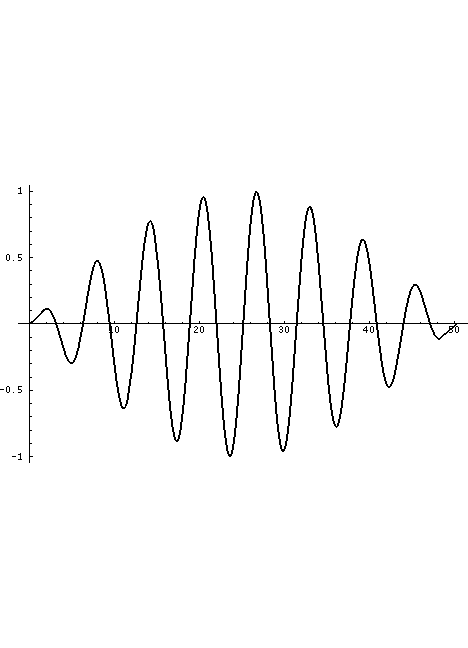
The volume flow through the glottis is roughly a triangular wave with a single discontinuity at closure which generally produces all harmonics of the fundamental glottal rate, falling off at roughly 12dB per octave with increasing harmonic frequency (remember, the dB scale is power-based with zero being an arbitrary reference power). This is what is displayed in the Waveform sub-panel.

Glottal Pulse Parameters

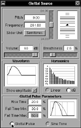
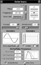
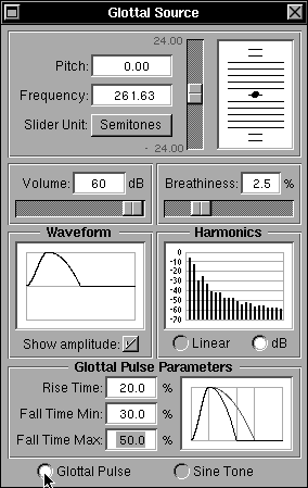
Fig 16a: Adjusting the rise and fall times for the glottal pulse

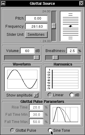
Fig 16b: Substituting sine wave excitation for the glottal pulse

The question of which artificial glottal pulse shape gives the most natural sounding voice has been a subject of research for decades. Our choice was the “Rosenburg B” waveform that is almost identical in shape to “Rosenberg C” as seen in the “Waveform” sub-panel. As an aid to visualisation, the Rosenberg C waveform comprises of a raised half sine wave joined smoothly to a quarter sine wave at twice the amplitude. The “Rosenberg B” is made of polynomial functions and, as noted, is almost indistinguishable. Both provide a smooth onset with a sharp termination (a single discontinuity in both first and second order derivatives) and the “B” version was experimentally judged by listeners to produce the most natural voice quality when substituted for the original glottal pulse in speech recomposed from a decomposition of natural speech (Rosenberg 1971) and has a slightly sharper offset so a little more high frequency content than the “C” version (which was a close second). A total of six artificial glottal pulse shapes were tested. A second experiment looked at the rise and fall times of the “C” waveform. The defaults chosen for Synthesizer are in the rise/fall region judged most natural in that experiment. The broader topic is usefully discussed in Witten (1982 pp 95-101) in connection with the excitation of resonance synthesisers which excite formant filters rather than a tube analogue. The fact remains that natural glottal excitation sounds better than even the best artificial glottal excitation, and also carries some speaker identification information.

Ideally, given enough knowledge and computational power, a proper aerodynamic model of the vibrating vocal folds would be used to excite the TRM. We would expect this to improve the naturalness of the voice quality significantly. Vocal fold/glottis modelling is a very active area of research. There is to be a conference on the topic in Marseille, France in August 2004 (Int Conf on Voice Physiology and Biomechanics August 18-20). Google on “vocal fold modeling” to gain access to a wide variety of research.

The parameters of the glottal pulse -- the rise and fall times -- can be varied as a percentage of the total glottal period using fields within the Glottal Pulse Parameters sub-panel at the bottom. The maximum duration of the fall time can also be set -- a value that is used during the wavetable calculations of the amplitude-varying glottal pulse -- effectively extending the fall period as the amplitude decreases, but limited by the maximum fall time set. The range for all three time parameters is limited from 5% to 50% of the total period. The parameters also control a nominal pulse shape display to the right of the same sub-panel with a greyed portion for the maximum. Figure 16a shows a situation in which the parameters have been changed from their default values.

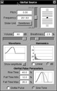
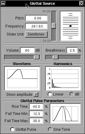
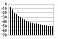
Fig 16c: Waveform and harmonics display

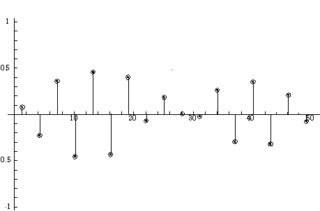
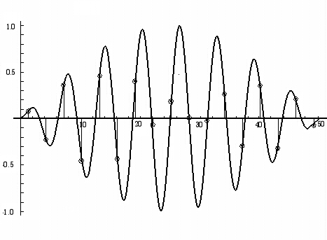
Immediately above the Glottal Parameters sub-panel lie the Waveform and Harmonics sub-panels which show the glottal pulse shape and the corresponding harmonic spectrum respectively. These respond to the glottal pulse parameter settings. If the radio buttons at the bottom of the main panel below the Glottal Pulse Parameters sub-panel are set to “Sine Tone” instead of “Glottal Pulse” the Waveform display changes to show a full cycle sine wave and the Harmonics display shows a single harmonic corresponding to the sine wave as shown in Figure 16b. The sine wave input can be used for test purposes, sweeping a single frequency through a range to examine the tube response to a pure tone. The Harmonics display can be swtiched from a dB display relative to the maximum harmonic to a linear display, using the radio buttons below the harmonics display, as shown in figure 16c.

Provided the “Show amplitude” check box just below the Waveform display is checked, the changes in shape and variation in fall time can be seen by changing the "Rise Time", "Fall Time Min." and "Fall Time Max." settings and varying the “Volume” control just above the Waveform display. The “Volume” control changes the amplitude of the pulse. The change in duration of the fall as the amplitude changes can be seen more easily by not checking the box, because then the displayed amplitude does not change according to the actual pulse amplitude.

Adjusting the pitch value

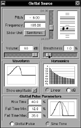
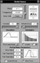
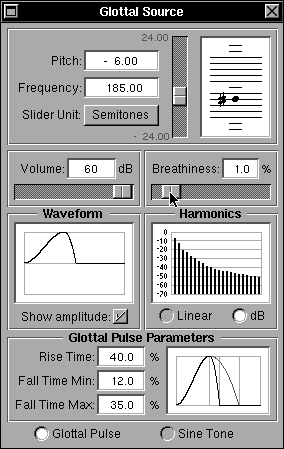
Fig 17a: Adjusting the pitch value: semintones

Fig 17b: Adjusting the pitch value: Cents

The frequency of the glottal pulse, or sine wave, is set at the top of the main panel using several controls plus a display of the musical note equivalent of the pitch. “Pitch” shows the TRM parameter value directly which nominally varies between +24 and -24, although this range does get slightly extended when necessary. “Frequency” shows the physical frequency corresponding to the pitch. Both fields may be entered directly, or the slider may be used to vary the pitch.Figure 17a shows a pitch adjustment away from the default value based on semitone adjustment

The “Slider Unit” pull-down allows “Semintones” or “Cents” to be selected as the units of change. The Cent is a logarithmic interpolation within a semi-tone and provides 100 logarithmic steps. Thus there are 1200 cents per octave since an octave is 12 semitones. If Cents are selected, then, as the pitch value is changed, the range of movement is restricted to one semi-tone and an up arrow or down arrow appears beside the musical note display according to whether the current setting is somewhat above or somewhat below the musical note displayed. Figure 17b shows the resulting change in the displays. The musical scale is calibrated to A = 440 Hz so that middle C comes out at 261.63 Hz rather than the old-fashioned 256 Hz. This is done to allow a singing voice to match modern musical instruments. A = 440 Hz is called “Concert Pitch”

“Breathy Voice”

The remaining control is “Breathiness” -- a slider and percentage display just below the musical note display. When the vocal folds are vibrating, they may not completely close at nominal closure for a variety of reasons. The commonest case is for female speech. A small triangle of the vocal fold gap remains open during the closure phase and allows air to leak through. This introduces a breathy noise (similar to light aspiration) during voiced sounds. The effect is characteristic of female speech and is called “breathy voice”. Readers, especially male readers, must be aware of the appeal of a “husky voice” which is an extreme version of this consistent sex marker. This is the main reason for including this control since one aim of the TRM is to emulate male, female and child voices accurately. Breathiness is an important parameter (along with tube length) for this exercise. The parameter can be varied from 0 to 10% of the excitation energy.

Explorations and the creation of .trm data files

Note: this section is only a sketch and needs expanding. A paper describing the generation of the current TRM posture database is currently in preparation, and will be an important reference for a revised and expanded section.

Creating TRM “postures”

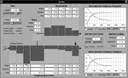
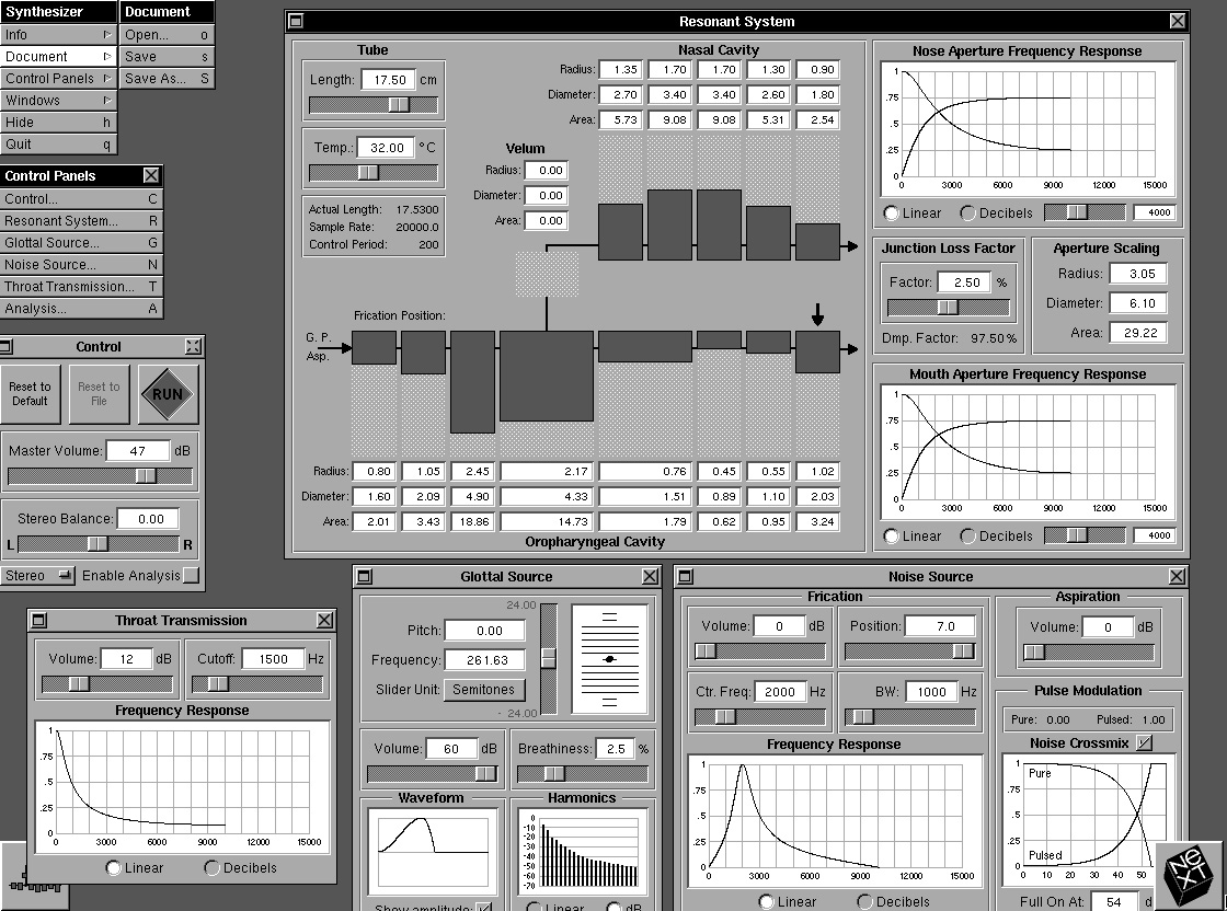
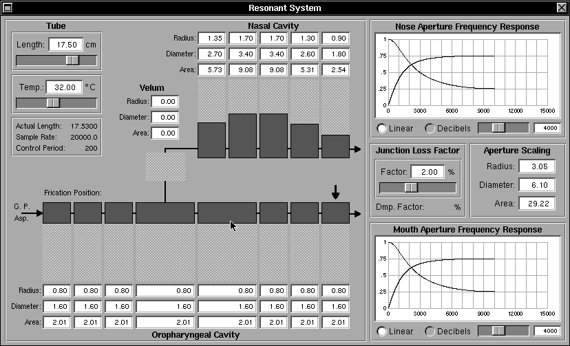
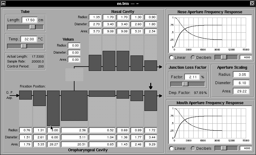
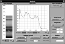
Fig 18a: The Resonant System panel showing oro-pharyngeal tube sections set up for an “ee-like” sound

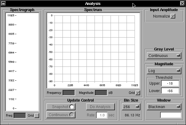
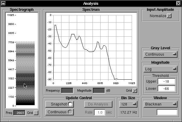
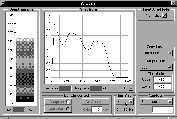
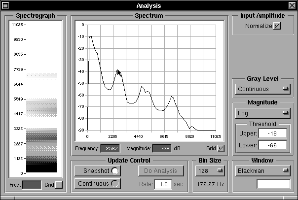
Fig 18b: The Analysis panel showing the broad band spectrum of the “ee-like” sound

To set up the TRM configuration for a sound only requires that you have some knowledge of articulatory phonetics and can interpret this knowledge as tube radii and the expected spectral output. Appendix A provides a set of data for the entire nominal postural structure of spoken English (additional detail such as co-articulation and some acoustic events are taken care of by the Monet/GnuSpeech parameter generation system). The regions, starting at r1 correspond to: 1 to 3 -- the pharynx; 4 -- the region either side of the velum; 5 -- the front part of the oral cavity behind the alveolar ridge; 6 -- the region around the alveolar ridge; 7 -- the region from the alveolar ridge to the teeth; and 8 -- the region from the teeth to the outside of the lips. Note that regions 4 and 5 are twice the length of the others, which are 1.6 cm long for a 16 cm vocal tract.

Lip opening affects r8. Jaw rotation affects r4 through r8. Tongue height (low to high) and position (back to front) affect r2 through r7 in a constrained way -- a high back vowel, for example, leads to narrowing of r2 through r4 and opening of r6/7. Exactly what effect it has on r5 will depend on the details of the articulation. A reasonable shape can be tried, preferably using articulatory data from the literature as a guide, and the effect can be checked by carrying out an analysis to determine the spectrum of the resulting sound. There is no precise data for the DRM control system, and the TRM control regions are not exactly aligned with these regions anyway. However, the match is close enough to get excellent results in synthetic speech with a low data rate compared to trying to control a 40 section tube model.

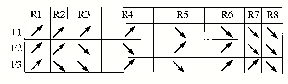
The paper “Real time articulatory synthesis ...” (Hill et al. 1995) includes a diagram showing how constrictions at the various DRM control regions affect the formants. It can be used as a guide when modifying the tube configurations to get a better spectral match to a given real sound. Vowel sounds are fairly straightforward. The data in Wells (1963) is a useful starting point for British English. The data published by Peterson and Barney (1952) is more appropriate to General American. Dealing with consonants, especially stop sounds, is more problematical since they may have no steady-state spectrum, or the spectrum may be masked by nasalisation, etc. However, knowing the apparent origins of the formant transitions can be a guide, as can listening to the resulting postures in continuous speech synthesis. Green's paper (1959) and Liberman's paper (1955) are helpful in this respect while Strevens (1960) gives some feel for the fricative characteristics. There is a wealth of literature, much of it from earlier times -- given the change in interest to synthesis by concatenated segments. The papers cited give an entry into the literature that is likely to be helpful, but the task is likely to prove difficult for any language in which the user's linguistic/phonetic knowledge is deficient.

Figure 18a shows the resonant system configured to produce a sound similar to “ee” in English. Figure 18b shows the broad band analysis of the resulting output. Note the low first formant, and relatively high formants 2 and 3, charateristic of this kind of sound. If a slightly different “ee-like” sound were required, the constrictions could be modified, knowing their effect in different DRMs from the paper quote above. Changes in pitch and breathiness could be tried and other parameters varied to listen to the effects of different conditions and see the spectral effects of changes that changed the spectrum. Then the .trm file could be saved (see next section), and read into the Monet system where the sound could be tried as part of continuous speech, listening to the result and performing a spectrographic analysis to understand the effect “in context”. This also highlights the fact that, for successful database creation, Synthesizer and Monet interact and must be used iteratively and in concert.

Note that only the parameters affecting the individual sound would be saved and transferred. Pitch is managed as a parameter separate from the TRM postures within the Monet system (except for micro-intonation special events) and a number of parameters are so-called “utterance rate” parameters, that do not vary from posture to posture (for example, tube length, temperature, pulse shape, mouth and nose aperture frequency responses, noise cross-mix, throat transmission, and junction loss factor).

Even the durations of the speech postures are outside the scope of Synthesizer. Posture durations control rhythm which is modelled as part of the Monet system along with the pitch variations that control intonation. Rhythm and intonation interact. Together they form prosody and, as previously noted, they directly and significantly affect meaning. A discussion of the issues is outside the scope of this manual, but some insight into the approach taken for the TextToSpeech Experimenter Kit may be gained from reports related to research at the U of Calgary and other places that underpins the system prosody (Halliday 1970; Hill 1978; Jassem, et al 1984; and Taube-Schock 1993).


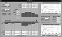
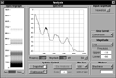
Fig 19a: The Resonant System panel showing oro-pharyngeal tube sections set up for an “oo-like” sound

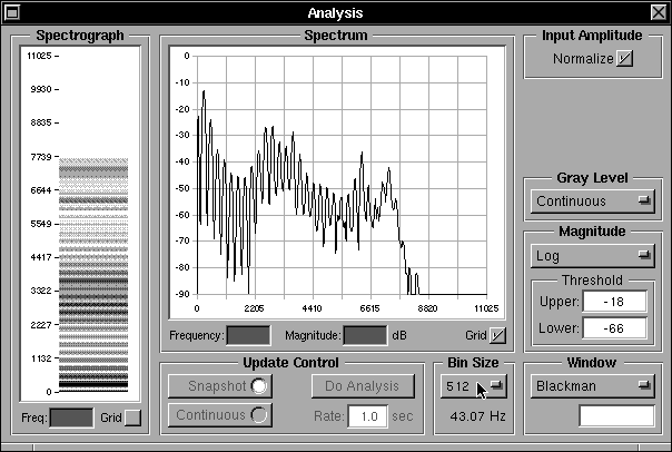
Fig 19b: The Analysis panel showing the broad band spectrum of the “oo-like” sound

Figures 19a and 19b show the same Resonant System and Analysis sub-system views as Figures 18a and 18b but for an “oo-like” English sound. The two configurations and analyses can be compared with each other, and with the data provided for the relevant postures used for text-to-speech synthesis that are listed in Appendix A.

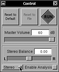
The various static controls, such as Glottal Source waveform, Throat Transmission and Mouth and Nose Aperture Frequency Response are generally best left at their default values, unless you have a particular objective in mind. The effects can be tried, out of interest. The one exception is the “Pitch” frequency. It is sometimes easier to hear the quality of the sound, for listening tests, with a value that is different to the default value. The author prefers a lower value.

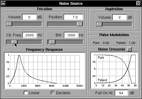
The Noise Crossmix is of use in sounds such as /z/, where the combination of vibrating vocal folds and vocal tract constriction produce both voicing, and a modulation of the fricative noise.

At present, the Tube length cannot be reduced below about 15 cm in the NeXT implementation because the computation rate is not sufficient to deal with shorter tube lengths (which means higher frequencies in the tube). Even when the system is not generating output, reducing the tube length too far will crash the system. Porting to modern systems with far higher computation rates and with DSP-like instructions available on the main processor, should eliminate this problem.


Saving .trm data

Fig 20: Document Menu

Figure 20 shows the Document menu. The three possible choices are to “Open” a .trm file previously created using Synthesizer, to “Save” the current working .trm file, or to create a new working file by selecting “Save As” to bring up a dialogue to set the new file name. The .trm files may be read into the Monet system to allow new postures to be created, saved, and entered into the Monet database without errors or unnecessary user actions.


Help facilities available

This on-line manual provides the only help facilities currently available. It needs to be upgraded so that individual topics can be searched and brought up conveniently within the Synthesizer system. This is not likely to happen in the near future!

Acknowledgements

The author wishes to acknowledge the fundamental work performed by Leonard Manzara in designing and implementing both the Tube Resonance Model itself and the excellent Synthesizer GUI that is the subject of this manual. The TRM exists both as 'C' software and as DSP56001 assembler code. At the time the model was first created, it was only by using a DSP as a co-processor that the tube model could run anywhere near real time. In fact, at that time, for shorter tube lengths which (perhaps counterintuitively) require a greater rate of computation, only tube lengths greater than around 15 cm could be computed in real time, even using the most appropriate DSP that was available. Craig Schock and the author were both involved in discussion, but the major player was Len, except for the idea of using 10 equal regions in the vocal tract, and combining the middle four into two pairs which was crucial to achieving real-time computation with a reasonably accurate version of the 8-region DRM control system.

References

ATAL, BS and SL HANAUER (1971) Speech analysis and synthesis by linear prediction of the speech wave, J Acoust Soc Amer, 50 (2), Aug, pp 637-633.

CARRE, R & S CHENNOUKH (1993) Vowel-Consonant-Vowel modeling by superposition of consonant closure on Vowel-to-Vowel gestures 3rd Seminar on Speech Production: Models and Data, Saybrook Point Inn May 11-13 1993

CARRE, R, S CHENNOUKH & M MRAYATI (1992) Vowel-consonant-vowel transitions: analysis, modeling and synthesis Proc ICSLP 92 (Int. Conf. of Spoken Language Processing), Banff, Alberta, pp 819-822

CARRE, R & MRAYATI, M (1994) Vowel transitions, vowel systems, and the Distinctive Region Model. in Levels in Speech Communication: Relations and Interactions. Elsevier: New York

CARRE, R, B LINDBLOM & P MACNEILAGE (1994) Acoustic contrast and the original of the human vowel space Acoust Soc Amer meeting, Cambridge MA, paper 3pSP

COOK, PR (1991) Identification of control parameters in an articulatory vocal tract model with applications to the synthesis of singing PhD Thesis, Stanford University, Dept of Electrical Eng, September

DUNN, HK (1950) The calculation of vowel resonances, and an electrical vocal tract J Acoust Soc Amer 22 pp 740-753

FANT, CGM & S PAULI (1974) Spatial characteristics of vocal tract resonance mod es. SCS 74 (Speech Communication Seminar, Stockholm, Aug 1-3 1974, pp 121-133

FANT, G (1956) On the predictability of formant levels and spectrum envelopes from formant frequencies. In For Roman Jakobson. Mouton: The Hague, 109-120

FANT, CGM (1960) Acoustic theory of speech production Mouton: The Hague

FANT, G & PAULI, S (1974) Spatial characteristics of vocal tract resonance models. Proceedings of the Stockholm Speech Communication Seminar, KTH, Stockholm, Sweden

FLANAGAN, JL (1972) Speech analysis, synthesis and perception Springer-Verlag: New York, ISBN 0-387-05561-4, 444 pp (Second Edition)

GREEN, PS (1959) Consonant-vowel transitions: a spectrographic study Travaux de l'Institut de Phonétique de Lund, (also in Studia Linguistica XII 1958 number 2) (available in the Essex University library, UK)

HALLIDAY, MAK (1970) A course in spoken English: intonation. Oxford University Press 134pp

HECKER, MHL (1962) - Studies of nasal consonants with an articulatory speech synthesiser. J Acoust Soc Amer 34, (2), February

HILL, DR (1978) Some results from a preliminary study of British English speech rhythm Research report 78/26/5, Dept of Comp Sci, U of Calgary, 24 pp

HILL, DR, MANZARA, L & TAUBE-SCHOCK, C-R (1995) Real-time articulatory speech-synthesis-by-rules. Proc. AVIOS '95 14th Annual International Voice Technologies Conf, San Jose, 12-14 September 1995, 27-44.

HILL, DR (1991) A conceptionary for speech and hearing in the context of machines and experimentation, Comp Sci Dept Report, 2nd edition 2004.

JASSEM, W, DR HILL & IH WITTEN (1984) Isochrony in English speech: its statistical validity and linguistic relevance in Intonation, Accent and Rhythm: studies in discourse phonology (D Gibbon & H Richter, eds), de Gruyter: Berlin & New York, ISBN 3-11-009832-6

LAWRENCE, W (1953) The synthesis of speech from signals which have a low information rate. In Communication Theory, Butterworth: London, 460-469

LAWRENCE, W (1954) The experimental synthesis of speech from parameters Signals Research and Development Establishment Report: Christchurch, UK

LIBERMAN, AM, P DELATTRE & FS COOPER (1955) Acoustic locii and transitional cues for 34 consonants J Acoust Soc Amer 27 (4), July

LIBERMAN, AM, INGEMANN, F, LISKER, L, DELATTRE, P & COOPER, FS (1959) Minimal rules for synthesising speech. J Acoust Soc Amer 31 (11), 1490-1499, Nov

MANZARA, L & DR HILL (2002) Pronunciation Guide (http://www.cpsc.ucalgary.ca/~hill/papers/monman/pronguid.html)

MARKEL, JD & AH GRAY (1976) Linear Prediction of Speech Springer-Verlag: New York, ISBN 3-540-07563-1

PETERSON, GE & BARNEY, HL (1952) Control methods used in the study of vowels J. Acoust Soc Amer 24 (3), 175-184, March. (Also Bell Monograph 1982)

POTTER, RK, GA KOPP & H GREEN (1947) Visible Speech Bell Telephone laboratories: Murray Hill, New Jersey (Dover edition 1966 LCCCN 65-23130, by which time Harriet Green had married George Kopp, so the authors were Potter, Kopp and Kopp)

ROSENBERG, AE (1971) Effect of glottal pulse shape on the quality of natural vowels J Acoust Soc Amer 49 583-590

TAUBE-SCHOCK, C-R (1993) Intonation for computer speech output MSc Thesis, Dept of Comp Sci, U of Calgary, September (available from University Microfilms) (note this is the same person as “Craig Schock”)

SHANNON, C (1948) The mathematical theory of communication Bell System Technical Journal, July & October

SMITH JO III (2004) Physical audio signal processing (URL: http://www-ccrma.stanford.edu/~jos/waveguide/) May

STEVENS, K, S KASOWSKI & CGM FANT (1953) An electrical analog of the vocal tract J Acoust Soc Amer 25 pp 743-742

STREVENS, P (1960) Spectra of fricative noises in human speech Language & Speech, 3 (1), Jan/Mar

TOLKIEN JRR (1966) The Return of the King George Allen & Unwin: London, UK (Unwin Paperbacks 1978 combined edition ISBN 0-04-823229-7, page 620: Pippin speaking to Gandalf as he is carried away from his encounter with the Palatír at Orthanc, read by David R. Hill; and analysed by Neal Reid under the NRC of Canada grant A5261)

WELLS, JC (1963) A study of the formants of the pure vowels of British English Progress Report, University College, London, UK, July

WHITFIELD, IC & EF EVANS (1965) Behaviour of Neurones in the unanaesthetised auditory cortex of the cat J. Neurophysiology 28, 655-672

WITTEN IH (1982) Principles of Computer Speech Academic Press: London, ISBN 0-12-760760-9, 286 pp


Appendix A: Derivation of and values for parameter data for Tube Resonance Model postures

(Note: This is the complete raw posture data contained in the GnuSpeech database. The Monet Manual, Appendix D contains the equivalent formant and timing data. Since the timing data varies between marked and unmarked versions of a given posture, each posture has two entries in that table.

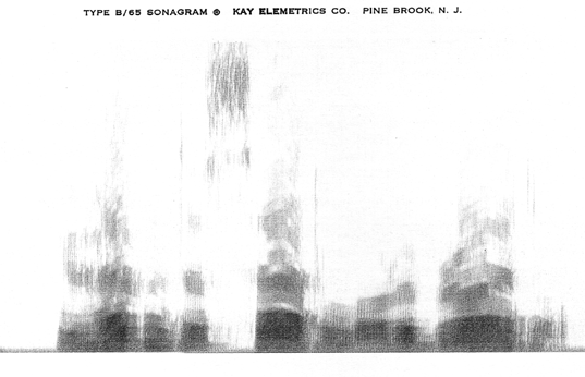
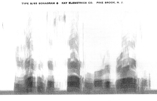
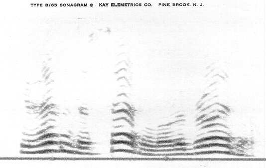
The TRM parameter data for the 65 or so articulatory postures that follow were experimentally derived during the last three months of 1994 by the author and Leonard Manzara working together. The details of the derivation should be included in a paper in preparation but involved: (1) analysis of real speech using a Kay Sonagraf and the Sonagram App on the NeXT computer; (2) use of real speech data from publications such as Wells' vowel data (Wells 1963); (3) the adjustment of the DRM regions and other parameters in the Tube Resonance Model using Synthesizer, starting from a knowledge of articulatory phonetics and the effect of constrictions in the eight DRM regions on formant frequencies; (4) the fact that the vocal tract has structural and dynamic constraints of the configurations that are possible; (5) the analysis of the TRM output using the Analysis sub-system of Synthesizer and a comparison of this with the analyses from real speech; and (6) the use of the Monet system to test the effectiveness of the postures derived, in continuous synthetic speech, by listening to a good variety of phonetic contexts. Development of the Monet context rules and rewrite rules proceeded in parallel, and the steps were iterated as necessary.

It will be noted that the r1 DRM region is always set to a 0.8 cm radius. In fact it probably need not have been included as a varying parameter because it really only determines the relative scale. Similar results could be obtained for all postures with different values of r1 leading to different, but geometrically similar values of the other 7 regions for each posture. This is presently an untested hypothesis, but one in which we have considerable confidence.

Region r1 corresponds to the first DRM region above the glottis. Region r8 corresponds to the last region before the mouth orifice. In some postures, the fricative spectral parameters (fricVol, fricPos, fricCF and fricBW) are set, with the fricative volume (fricVol) at zero. This is because the particular posture is associated with a fricative noise burst in which the fricative volume is controlled by a special event parameter profile rather than the regular parameter control using the fricative volume value. The fricative volume parameter settings are generally rather low. The noise balances within the TRM implementation need some attention. It causes some problems in the parameter displays within the Monet system because the values are hardly visible at values which give acceptable output energy. This and the small range to work with also makes adjusting fricatives, especially voiced fricatives during database creation somewhat tricky, especially for the placement and volume of special events.

The velum “closed” value default is 0.1 -- very slightly open. The same is true of closure for /t,d,k,g/ at their points of articulation (r6), /k,g/ (r5), and lip closure for /b,p/ (associated with r8, though this is a bit of a fudge -- it may be better to close the mouth orifice and leave r8 to be manipulated independently; mouth closure could be substituted for the r1 parameter to keep the number of dynamically variable parameters the same). The slight opening avoids some slight artifacts without affecting the articulations.

It is important to realise that perceiving TRM postures is both static and dynamic. Vowels, which can be represented as a stand-alone steady state sound without losing any of their identity, can be heard when the TRM posture (articulation) is appropriately set up, though the ear and brain soon become habituated to the noise which begins to lose its identity. Short bursts of the sound are more convincing, but still lack the dynamic variation of real speech. However, when you come to steady state consonant postures (articulations), many of the cues we use in perceiving them are simply absent because the cues are dynamic (changes in formant frequency, or fricative characteristics as the sound approaches and leaves the posture, and noise bursts). Some consonant postures preclude any sound because the oro-pharyngeal and nasal passages are completely closed, though some sound may escape for a short time through the throat tissues if the vocal folds are vibrating -- so called “voice bar” in the Visible Speech terminology. If the closure is maintained, the flexible parts of the tract fill up and air can no longer flow, so the vocal folds stop vibrating. Consonant postures can only be tested as part of continuous speech, which is what we had to do. The locus theory of consonant perception (Liberman 1955, for example) derives from this essential basic fact. To the extent that such locii (the frequencies from which or to which formant transitions appear to move in speech spectrograms) exist, they are related to the postures associated with the consonants. The phenomenon of co-articulation -- the influence of context on the actual configuration in continuous speech -- ensures that there are no fixed locii for consonants any more than there are fixed formant combinations for vowels. However, there is a grain of truth in the idea of consonant locii. The GnuSpeech system context rules are designed to allow such co-articulation effects to be included. Green (1959) provides a comprehensive spectrographic study of consonant-vowel transitions.

The pronunciations associated with the posture symbols below, which were designed to be mnemonic and easily typed, have been rendered in terms of both the International Phonetic Association and Websters phonetic symbols, together with other helpful information, in an on-line pronunciation guide (Manzara & Hill 2002). Note that only one version of each posture is provided. The marked, unmarked and other (e.g. syllabic) versions have the same TRM parameter values. Only the durations differ. Durations are relevant to the Monet/GnuSpeech level rather than the TRM level. Also, as already noted, some acoustic characteristics (for example, bursts of aspiration or fricative noise, and co-articulation effects) of the sounds are managed by the rules and prototypes in the Monet/GnuSpeech system and are, as far as the TRM is concerned “hidden”.

Phone
Parameters
microInt glotVol aspVol fricVol fricPos fricCF fricBW velum
r1 r2 r3 r4 r5 r6 r7 r8
# 0.0 0.0 0.0 0.0 5.5 2500.0 500.0 0.1
0.8 0.89 0.99 0.81 0.76 1.05 1.23 0.01
^ 0.0 0.0 0.0 0.0 5.5 2500.0 500.0 0.1
0.8 0.89 0.99 0.81 0.76 1.05 1.23 0.01
a 0.0 60.0 0.0 0.0 5.5 2500.0 500.0 0.1
0.8 0.65 0.65 0.65 1.31 1.23 1.31 1.67
aa 0.0 60.0 0.0 0.0 5.5 2500.0 500.0 0.1
0.8 0.65 0.84 1.15 1.31 1.59 1.59 2.61
ah 0.0 60.0 0.0 0.0 5.5 2500.0 500.0 0.1
0.8 0.65 0.45 0.94 1.1 1.52 1.46 2.45
an 0.0 60.0 0.0 0.0 5.5 2500.0 500.0 1.5
0.8 0.52 0.45 0.79 1.49 1.67 1.02 1.59
ar 0.0 60.0 0.0 0.0 5.5 2500.0 500.0 0.1
0.8 0.52 0.45 0.79 1.49 1.67 1.02 1.59
aw 0.0 60.0 0.0 0.0 5.5 2500.0 500.0 0.1
0.8 1.1 0.94 0.42 1.49 1.67 1.78 1.05
b -2.0 43.5 0.0 0.0 7.0 2000.0 700.0 0.1
*0.8 0.89 0.76 1.28 1.8 0.99 0.84 0.1
ch -2.0 0.0 0.0 0.0 5.6 2500.0 2600.0 0.1
0.8 1.36 1.74 1.87 0.94 0.0 0.79 0.79
d *-2.0 43.5 0.0 0.0 6.7 4500.0 2000.0 0.1
0.8 1.31 1.49 1.25 0.76 0.1 1.44 1.3
dh -1.0 54.0 0.0 0.25 6.0 4400.0 4500.0 0.1
0.8 1.2 1.5 1.35 1.2 1.2 0.4 1.0
e 0.0 60.0 0.0 0.0 5.5 2500.0 500.0 0.1
0.8 0.68 1.12 1.70 1.39 1.07 1.05 2.06
ee 0.0 60.0 0.0 0.0 5.5 2500.0 500.0 0.1
0.8 1.67 1.91 1.99 0.81 0.495 0.73 1.49
er 0.0 60.0 0.0 0.0 5.5 2500.0 500.0 0.1
0.8 0.89 0.99 0.81 0.76 1.04 1.23 1.12
f -1.0 0.0 0.0 0.5 7.0 3300.0 1000.0 0.1
0.8 0.89 0.99 0.81 0.76 0.89 0.84 0.5
g *-2.0 43.5 0.0 0.0 4.7 2000.0 2000.0 0.1
0.8 1.7 1.3 0.99 0.1 1.07 0.73 1.49
gs 0.0 0.0 0.0 0.0 5.5 2500.0 500.0 0.1
0.8 0.8 0.8 0.8 0.8 0.8 0.8 0.8
h *0.0 0.0 10.0 0.0 5.5 2500.0 500.0 0.1
0.8 0.8 0.8 0.8 0.8 0.8 0.8 0.8
Phone
Parameters
microInt glotVol aspVol fricVol fricPos fricCF fricBW velum
r1 r2 r3 r4 r5 r6 r7 r8
hh 0.0 0.0 10.0 0.0 1.0 1000.0 1000.0 0.1
0.8 0.24 0.4 0.81 0.76 1.05 1.23 1.12
hv 0.0 42.0 10.0 0.0 5.5 2500.0 500.0 0.1
0.8 0.8 0.8 0.8 0.8 0.8 0.8 0.8
i 0.0 60.0 0.0 0.0 5.5 2500.0 500.0 0.1
0.8 1.05 1.57 1.75 0.94 0.68 0.79 1.12
in 0.0 60.0 0.0 0.0 5.5 2500.0 500.0 1.5
0.8 0.65 0.84 1.15 1.31 1.59 1.59 2.61
j -2.0 48.0 0.0 0.0 5.6 2500.0 2600.0 0.1
0.8 1.36 1.74 1.87 0.94 0.0 0.79 0.79
k -10.0 0.0 0.0 0.0 4.7 2000.0 2000.0 0.1
0.8 1.7 1.3 0.99 0.1 1.07 0.73 1.49
l 0.0 60.0 0.0 0.0 5.5 2500.0 500.0 0.1
0.8 0.89 1.1 0.97 0.89 0.34 0.29 1.12
ll 0.0 60.0 0.0 0.0 5.5 2500.0 500.0 0.1
0.8 0.63 0.47 0.65 1.54 0.45 0.26 1.05
m 0.0 60.0 0.0 0.0 5.5 2500.0 500.0 0.5
0.8 0.89 0.76 1.28 1.8 0.99 *0.84 0.1
n 0.0 60.0 0.0 0.0 5.5 2500.0 500.0 0.5
0.8 1.31 1.49 1.25 1.0 0.05 1.44 1.31
ng 0.0 60.0 0.0 0.0 5.5 2500.0 500.0 0.5
0.8 1.7 1.3 0.99 0.1 1.07 0.73 1.49
o 0.0 60.0 0.0 0.0 5.5 2500.0 500.0 0.1
0.8 1.0 0.93 0.6 1.27 1.83 1.97 1.12
oh 0.0 60.0 0.0 0.0 5.5 2500.0 500.0 0.1
0.8 0.89 0.99 0.81 0.76 1.05 1.23 1.12
on 0.0 60.0 0.0 0.0 5.5 2500.0 500.0 1.5
0.8 1.0 0.93 0.6 1.27 1.83 1.97 1.12
ov 0.0 60.0 0.0 0.0 5.5 2500.0 500.0 0.1
0.8 0.89 0.99 0.81 0.76 1.05 1.23 1.12
p -10.0 0.0 0.0 0.0 7.0 2000.0 700.0 0.1
0.8 0.89 0.76 1.28 1.8 0.99 0.84 0.1
ph -1.0 0.0 0.0 24 7.0 864.0 3587.0 0.1
0.8 0.89 0.99 0.81 0.6 0.52 0.71 0.24
q 0.0 0.0 0.0 0.0 5.5 2500.0 500.0 0.1
0.8 0.89 0.99 0.81 0.76 1.05 1.23 0.01
qc -2.0 0.0 0.0 0.0 5.6 2500.0 2600 0.1
0.8 1.36 1.74 1.87 0.94 0.1 0.79 0.79
qk -10.0 0.0 0.0 0.0 4.7 2000.0 2000.0 0.1
0.8 1.7 1.3 0.99 0.1 1.07 0.73 1.49
Phone
Parameters
microInt glotVol aspVol fricVol fricPos fricCF fricBW velum
r1 r2 r3 r4 r5 r6 r7 r8
qp -10.0 0.0 0.0 0.0 7.0 2000.0 700.0 0.1
0.8 0.89 0.76 1.28 1.8 0.99 0.84 0.1
qs 0.0 0.0 0.0 0.0 5.8 5500.0 500.0 0.1
0.8 1.31 1.49 1.25 0.9 0.2 0.4 1.31
qt -10.0 0.0 0.0 0.0 7.0 4500.0 2000.0 0.1
0.8 1.31 1.49 1.25 0.76 0.1 1.44 1.31
qz -1.0 0.0 0.0 0.0 5.8 5500.0 500.0 0.1
0.8 1.31 1.49 1.25 0.9 0.2 0.6 1.31
r 0.0 60.0 0.0 0.0 5.5 2500.0 500.0 0.1
0.8 1.31 0.73 1.07 2.12 0.47 1.78 0.65
rr 0.0 60.0 0.0 0.0 5.5 2500.0 500.0 0.1
0.8 1.31 0.73 1.31 2.12 0.63 1.78 0.65
s 0.0 0.0 0.0 0.8 5.8 5500 500.0 0.1
0.8 1.31 1.49 1.25 0.9 0.2 0.4 1.31
sh 0.0 0.0 0.0 0.4 5.6 2500.0 2600.0 0.1
0.8 1.36 1.74 1.87 0.94 0.37 0.79 0.79
t -10.0 0.0 0.0 0.0 7.0 4500.0 2000.0 0.1
0.8 1.31 1.49 1.25 0.76 0.1 1.44 1.31
th 0.0 0.0 0.0 0.0 0.25 6.0 4400.0 4500.0
0.8 1.2 1.5 1.35 1.2 1.2 0.4 1.0
u 0.0 60.0 0.0 0.0 5.5 2500.0 500.0 0.1
0.8 0.63 0.6 0.71 1.12 1.93 1.52 0.63
uh 0.0 60.0 0.0 0.0 5.5 2500.0 500.0 0.1
0.8 0.89 0.99 0.81 0.76 1.05 1.23 1.12
un 0.0 60.0 0.0 0.0 5.5 2500.0 500.0 1.5
0.8 0.89 0.99 0.81 0.755 1.05 1.23 1.12
uu 0.0 60.0 0.0 0.0 5.5 2500.0 500.0 0.1
0.8 1.91 1.44 0.6 1.02 1.33 1.56 0.55
v -1.0 54.0 0.0 0.2 7.0 3300.0 1000.0 0.1
0.8 0.89 0.99 0.99 0.81 0.76 0.89 0.5
w 0.0 60.0 0.0 0.0 5.5 2500.0 500.0 0.1
0.8 1.91 1.44 0.6 1.02 1.33 1.56 0.55
x 0.0 0.0 0.0 0.5 2.0 1770.0 900.0 0.1
0.8 1.7 1.3 0.4 0.99 1.07 0.73 1.49
y 0.0 60.0 0.0 0.0 5.5 2500.0 500.0 0.25
0.8 1.67 1.91 1.99 0.63 0.29 0.58 1.49
z *-1.0 54.0 0.0 0.8 5.8 5500.0 500.0 0.1
0.8 1.31 1.49 1.25 0.9 0.2 0.6 1.31
zh -1.0 54.0 0.0 0.4 5.6 2500.0 2600.0 0.1
0.8 1.36 1.74 1.87 0.94 0.37 0.79 0.79
Phone
Parameters
microInt glotVol aspVol fricVol fricPos fricCF fricBW velum
r1 r2 r3 r4 r5 r6 r7 r8

Appendix B: GNU Free Documentation Licence

GNU Free Documentation License

Version 1.1, March 2000

Copyright (C) 2000  Free Software Foundation, Inc.
59 Temple Place, Suite 330, Boston, MA  02111-1307  USA
Everyone is permitted to copy and distribute verbatim copies
of this license document, but changing it is not allowed.

0. PREAMBLE

The purpose of this License is to make a manual, textbook, or other written document "free" in the sense of freedom: to assure everyone the effective freedom to copy and redistribute it, with or without modifying it, either commercially or noncommercially. Secondarily, this License preserves for the author and publisher a way to get credit for their work, while not being considered responsible for modifications made by others.

This License is a kind of "copyleft", which means that derivative works of the document must themselves be free in the same sense. It complements the GNU General Public License, which is a copyleft license designed for free software.

We have designed this License in order to use it for manuals for free software, because free software needs free documentation: a free program should come with manuals providing the same freedoms that the software does. But this License is not limited to software manuals; it can be used for any textual work, regardless of subject matter or whether it is published as a printed book. We recommend this License principally for works whose purpose is instruction or reference.

1. APPLICABILITY AND DEFINITIONS

This License applies to any manual or other work that contains a notice placed by the copyright holder saying it can be distributed under the terms of this License. The "Document", below, refers to any such manual or work. Any member of the public is a licensee, and is addressed as "you".

A "Modified Version" of the Document means any work containing the Document or a portion of it, either copied verbatim, or with modifications and/or translated into another language.

A "Secondary Section" is a named appendix or a front-matter section of the Document that deals exclusively with the relationship of the publishers or authors of the Document to the Document's overall subject (or to related matters) and contains nothing that could fall directly within that overall subject. (For example, if the Document is in part a textbook of mathematics, a Secondary Section may not explain any mathematics.) The relationship could be a matter of historical connection with the subject or with related matters, or of legal, commercial, philosophical, ethical or political position regarding them.

The "Invariant Sections" are certain Secondary Sections whose titles are designated, as being those of Invariant Sections, in the notice that says that the Document is released under this License.

The "Cover Texts" are certain short passages of text that are listed, as Front-Cover Texts or Back-Cover Texts, in the notice that says that the Document is released under this License.

A "Transparent" copy of the Document means a machine-readable copy, represented in a format whose specification is available to the general public, whose contents can be viewed and edited directly and straightforwardly with generic text editors or (for images composed of pixels) generic paint programs or (for drawings) some widely available drawing editor, and that is suitable for input to text formatters or for automatic translation to a variety of formats suitable for input to text formatters. A copy made in an otherwise Transparent file format whose markup has been designed to thwart or discourage subsequent modification by readers is not Transparent. A copy that is not "Transparent" is called "Opaque".

Examples of suitable formats for Transparent copies include plain ASCII without markup, Texinfo input format, LaTeX input format, SGML or XML using a publicly available DTD, and standard-conforming simple HTML designed for human modification. Opaque formats include PostScript, PDF, proprietary formats that can be read and edited only by proprietary word processors, SGML or XML for which the DTD and/or processing tools are not generally available, and the machine-generated HTML produced by some word processors for output purposes only.

The "Title Page" means, for a printed book, the title page itself, plus such following pages as are needed to hold, legibly, the material this License requires to appear in the title page. For works in formats which do not have any title page as such, "Title Page" means the text near the most prominent appearance of the work's title, preceding the beginning of the body of the text.

2. VERBATIM COPYING

You may copy and distribute the Document in any medium, either commercially or noncommercially, provided that this License, the copyright notices, and the license notice saying this License applies to the Document are reproduced in all copies, and that you add no other conditions whatsoever to those of this License. You may not use technical measures to obstruct or control the reading or further copying of the copies you make or distribute. However, you may accept compensation in exchange for copies. If you distribute a large enough number of copies you must also follow the conditions in section 3.

You may also lend copies, under the same conditions stated above, and you may publicly display copies.

3. COPYING IN QUANTITY

If you publish printed copies of the Document numbering more than 100, and the Document's license notice requires Cover Texts, you must enclose the copies in covers that carry, clearly and legibly, all these Cover Texts: Front-Cover Texts on the front cover, and Back-Cover Texts on the back cover. Both covers must also clearly and legibly identify you as the publisher of these copies. The front cover must present the full title with all words of the title equally prominent and visible. You may add other material on the covers in addition. Copying with changes limited to the covers, as long as they preserve the title of the Document and satisfy these conditions, can be treated as verbatim copying in other respects.

If the required texts for either cover are too voluminous to fit legibly, you should put the first ones listed (as many as fit reasonably) on the actual cover, and continue the rest onto adjacent pages.

If you publish or distribute Opaque copies of the Document numbering more than 100, you must either include a machine-readable Transparent copy along with each Opaque copy, or state in or with each Opaque copy a publicly-accessible computer-network location containing a complete Transparent copy of the Document, free of added material, which the general network-using public has access to download anonymously at no charge using public-standard network protocols. If you use the latter option, you must take reasonably prudent steps, when you begin distribution of Opaque copies in quantity, to ensure that this Transparent copy will remain thus accessible at the stated location until at least one year after the last time you distribute an Opaque copy (directly or through your agents or retailers) of that edition to the public.

It is requested, but not required, that you contact the authors of the Document well before redistributing any large number of copies, to give them a chance to provide you with an updated version of the Document.

4. MODIFICATIONS

You may copy and distribute a Modified Version of the Document under the conditions of sections 2 and 3 above, provided that you release the Modified Version under precisely this License, with the Modified Version filling the role of the Document, thus licensing distribution and modification of the Modified Version to whoever possesses a copy of it. In addition, you must do these things in the Modified Version:

  • A. Use in the Title Page (and on the covers, if any) a title distinct from that of the Document, and from those of previous versions (which should, if there were any, be listed in the History section of the Document). You may use the same title as a previous version if the original publisher of that version gives permission.
  • B. List on the Title Page, as authors, one or more persons or entities responsible for authorship of the modifications in the Modified Version, together with at least five of the principal authors of the Document (all of its principal authors, if it has less than five).
  • C. State on the Title page the name of the publisher of the Modified Version, as the publisher.
  • D. Preserve all the copyright notices of the Document.
  • E. Add an appropriate copyright notice for your modifications adjacent to the other copyright notices.
  • F. Include, immediately after the copyright notices, a license notice giving the public permission to use the Modified Version under the terms of this License, in the form shown in the Addendum below.
  • G. Preserve in that license notice the full lists of Invariant Sections and required Cover Texts given in the Document's license notice.
  • H. Include an unaltered copy of this License.
  • I. Preserve the section entitled "History", and its title, and add to it an item stating at least the title, year, new authors, and publisher of the Modified Version as given on the Title Page. If there is no section entitled "History" in the Document, create one stating the title, year, authors, and publisher of the Document as given on its Title Page, then add an item describing the Modified Version as stated in the previous sentence.
  • J. Preserve the network location, if any, given in the Document for public access to a Transparent copy of the Document, and likewise the network locations given in the Document for previous versions it was based on. These may be placed in the "History" section. You may omit a network location for a work that was published at least four years before the Document itself, or if the original publisher of the version it refers to gives permission.
  • K. In any section entitled "Acknowledgements" or "Dedications", preserve the section's title, and preserve in the section all the substance and tone of each of the contributor acknowledgements and/or dedications given therein.
  • L. Preserve all the Invariant Sections of the Document, unaltered in their text and in their titles. Section numbers or the equivalent are not considered part of the section titles.
  • M. Delete any section entitled "Endorsements". Such a section may not be included in the Modified Version.
  • N. Do not retitle any existing section as "Endorsements" or to conflict in title with any Invariant Section.

If the Modified Version includes new front-matter sections or appendices that qualify as Secondary Sections and contain no material copied from the Document, you may at your option designate some or all of these sections as invariant. To do this, add their titles to the list of Invariant Sections in the Modified Version's license notice. These titles must be distinct from any other section titles.

You may add a section entitled "Endorsements", provided it contains nothing but endorsements of your Modified Version by various parties--for example, statements of peer review or that the text has been approved by an organization as the authoritative definition of a standard.

You may add a passage of up to five words as a Front-Cover Text, and a passage of up to 25 words as a Back-Cover Text, to the end of the list of Cover Texts in the Modified Version. Only one passage of Front-Cover Text and one of Back-Cover Text may be added by (or through arrangements made by) any one entity. If the Document already includes a cover text for the same cover, previously added by you or by arrangement made by the same entity you are acting on behalf of, you may not add another; but you may replace the old one, on explicit permission from the previous publisher that added the old one.

The author(s) and publisher(s) of the Document do not by this License give permission to use their names for publicity for or to assert or imply endorsement of any Modified Version.

5. COMBINING DOCUMENTS

You may combine the Document with other documents released under this License, under the terms defined in section 4 above for modified versions, provided that you include in the combination all of the Invariant Sections of all of the original documents, unmodified, and list them all as Invariant Sections of your combined work in its license notice.

The combined work need only contain one copy of this License, and multiple identical Invariant Sections may be replaced with a single copy. If there are multiple Invariant Sections with the same name but different contents, make the title of each such section unique by adding at the end of it, in parentheses, the name of the original author or publisher of that section if known, or else a unique number. Make the same adjustment to the section titles in the list of Invariant Sections in the license notice of the combined work.

In the combination, you must combine any sections entitled "History" in the various original documents, forming one section entitled "History"; likewise combine any sections entitled "Acknowledgements", and any sections entitled "Dedications". You must delete all sections entitled "Endorsements."

6. COLLECTIONS OF DOCUMENTS

You may make a collection consisting of the Document and other documents released under this License, and replace the individual copies of this License in the various documents with a single copy that is included in the collection, provided that you follow the rules of this License for verbatim copying of each of the documents in all other respects.

You may extract a single document from such a collection, and distribute it individually under this License, provided you insert a copy of this License into the extracted document, and follow this License in all other respects regarding verbatim copying of that document.

7. AGGREGATION WITH INDEPENDENT WORKS

A compilation of the Document or its derivatives with other separate and independent documents or works, in or on a volume of a storage or distribution medium, does not as a whole count as a Modified Version of the Document, provided no compilation copyright is claimed for the compilation. Such a compilation is called an "aggregate", and this License does not apply to the other self-contained works thus compiled with the Document, on account of their being thus compiled, if they are not themselves derivative works of the Document.

If the Cover Text requirement of section 3 is applicable to these copies of the Document, then if the Document is less than one quarter of the entire aggregate, the Document's Cover Texts may be placed on covers that surround only the Document within the aggregate. Otherwise they must appear on covers around the whole aggregate.

8. TRANSLATION

Translation is considered a kind of modification, so you may distribute translations of the Document under the terms of section 4. Replacing Invariant Sections with translations requires special permission from their copyright holders, but you may include translations of some or all Invariant Sections in addition to the original versions of these Invariant Sections. You may include a translation of this License provided that you also include the original English version of this License. In case of a disagreement between the translation and the original English version of this License, the original English version will prevail.

9. TERMINATION

You may not copy, modify, sublicense, or distribute the Document except as expressly provided for under this License. Any other attempt to copy, modify, sublicense or distribute the Document is void, and will automatically terminate your rights under this License. However, parties who have received copies, or rights, from you under this License will not have their licenses terminated so long as such parties remain in full compliance.

10. FUTURE REVISIONS OF THIS LICENSE

The Free Software Foundation may publish new, revised versions of the GNU Free Documentation License from time to time. Such new versions will be similar in spirit to the present version, but may differ in detail to address new problems or concerns. See http://www.gnu.org/copyleft/.

Each version of the License is given a distinguishing version number. If the Document specifies that a particular numbered version of this License "or any later version" applies to it, you have the option of following the terms and conditions either of that specified version or of any later version that has been published (not as a draft) by the Free Software Foundation. If the Document does not specify a version number of this License, you may choose any version ever published (not as a draft) by the Free Software Foundation.

--------------end of Free Documentation Licence copy------

Footnotes

1. The Synthesizer Tube Resonance Model (TRM, waveguide model, "tube model or transmission-line analog) vocal tract that forms the basis of the GnuSpeech text-to-speech system was designed and programmed by Leonard Manzara whilst at Trillium Sound Research Incorporated. The Distinctive Region Model control system which is used to control the TRM is based on research by CGM Fant and his colleagues at the Stockholm Royal Institute of Technology Speech Technology Laboratory (Fant & Pauli 1974) and by Rénèe Carré at Télécom Paris (Carré, Chennoukh & Mrayati 1992). (back)

2. Phonemes only have meaning in the context of a specified language. The sounds produced in speaking the language are termed "phones". These sounds may be grouped into classes or categories, two sounds belonging in the same category if they never distinguish two words in the language. The categories are the phonemes of the language, each containing many different allophones, the variation between which is insignificant as far as meaning is concerned. Thus phonemes are functionally defined abstract categories, and are specific to a language. The topic and related concepts are discussed in more detail in the author's “Conceptionary”.
(back to “Background to Synthesizer”) (back to “Spectrograms”)

3. The underlying control model used for the tube-model is derived from research carried out at the Ecole Nationale Supérieur des Télécommunication (ENST), Laboratoire de Traitment et Communication de l'Information (LCTI) (Department of Signals), in Paris, by Dr. Réné Carré. This work in turn built on earlier work by Fant and his colleagues at the Speech Technology Laboratory, at KTH in Stockholm. Background on this research and the authors' developments from it are provided in Hill, Manzara and Taube-Schock (1995) (back)


Please email any comments or questions about this manual to the author (David Hill)

Page last updated 08-07-27.