Table of Contents

Best-first Search uses an evalution function to estimate the lowest cost among the paths to the next node.  A evaluation function returns a number purporting to describe the desirability of expanding the node.  Best-first Search takes two basic approaches.  The first one tries to expand the node closest to the goal (Greedy Search).  The second one tries to expand the node on the least-cost solution path (A* Search).
 

1.1  Greedy Search 

Greedy search is one of the simpliest best-first strategies which minimize the estimated cost.  It applies the heuristic function which estimated cost of the cheapest path from the state at node n to a goal state.  To help a better understanding of the greedy search algorithm, we investigate the
route-f inding problem.  Route finding problems applies the heuristic straight line distance function to get to the goal.

Figure 1.1   A state space with an initial state A and a final state I.  Arcs between any two states show the cost of  the  path.  For example the cost  from A to B is 75.

State	h(n)
A	366
B	374
C	329
D	244
E	253
F	178
G	193
H	98
I	0

Figure 1.2  Shows the resulting values of the heuristic function at each of the states.

 

According to the example given, we can find the cheapest path by following the statistics provided in figure 1.2.  The following is the progress of a greedy search to find the path from A to I.  With the straight-line heuristic, the fist node to expanded from A will be E because it is closer to I than either B or C.  The next node to expanded will be F, because it is closest.  F in turn generates I, which is our goal.  The resulting path is A-E-F-I with the total cost of 431.  However, this is not the optimal solution because there is a flaw in this algorithm. First of all, it will always pick the shortest straight line distance to the goal (in our case, from E, we picked to go to F-I instead of going to G-H-I since it is shorter in comparsion).  However, the actual path to the next node to the goal might be longer resulting higher cost.  In addition, this algorithm might give a incompleted solution.  It can start down an infinite path and never return to the try other possibilities.  In figure 1.3,   the straight line distance from A-D is shorter than from C-D.  Therefore the algorithm would pick A instead of C without considering if there's a actual path from node A to D. 
 

Figure 1.3  The straight line distance from A-D is shorter than from C-D.

 

1.2  A* Search

Although Greedy search cuts the search cost considerably, it does not give a optimal solution.  Combining the heuristic search from the Greedy search as well as the Uniform-cost search, the problem can be eliminated.  Uniform-cost search expands the least-cost leaf node first.  It is complete, and unlike heuristic search, is optimal.  Thus, if we are trying to find the cheapest solution, we can first try the node with the lowest value from the A* search.  We can also put a restriction to choose an function that never overestimates the cost to reach the goal using admissible heuristic.

The accuracy of the previous algorithms is dependent of the heuristic functions.  An example of a heuristic seen earlier is the straight-line distance for route-finding problems.  A heuristic function not only returns the estimated cost of the cheapest solution but also should never overestimate the cost to reach the goal.  Heuristic functions inherit such characteristics are known as admissible heuristics.  Heuristic function is basically an intelligence way to solve a given problem. Figure 4.7 below is one of many old heuristic search problems.  It is known as the 8-puzzle.

Start State

Goal State

Fig. 4.7  A typical instance of the 8-puzzle

There are three possible sets of moves depending on the initial location of an empty space.  If the empty space is in the corner, there are two; when it is along an edge there are three; and when it is in the center there are four.  A solution of 20 moves is typical for this puzzle but this varies depending on the initial state.  The number of states required for a depth of 20 would be about 3²⁰ = 3.5 x 10⁹.  If the repeated states are being kept track of, the number of states would be reduced drastically because there are only 9! = 362,000 possible arrangements.  This number is still significantly high .  Therefore finding a good heuristic is a must in order to reduce the number of arrangements.  The following heuristics are taken from the Artificial Intelligence: A Modern Approach, Stuart Russell & Peter Norvig - 1995.
 

• h₁ = the number of tiles that are in the wrong position.  For Figure 4.7, seven of the eight tiles are out of position, so the start state would have h₁ = 7.  h₁ is an admissible heuristic, because it is clear that any tile that is out of place must be moved at least once.
• h₂ = the sum of the distances of the tiles from their goal positions.  Because tiles cannot move along diagonals, the distance we will count is the sum of the horizontal and vertical distances.  This is sometimes called the city block distance or Manhattan distance.  h₂ is also admissible, because any move can only move one tile one step closer to the goal.  Tiles 1 to 8 in the start state give a Manhattan distance of

h₂ = 2 + 3 + 3 + 2 + 4 + 2 + 0 + 2 = 18

2.1  Inventing Heuristic Functions

We now have two heuristics available to choose from.  The decision now is to decide which heuristic function is better.  One suggested method for choosing a heuristic among the givens is by comparing the effective branching factor b*.  The equation to derive the effective branching factor is given as

N = 1 + b^* + (b^*)² + ... + (b^*)^d

where N = number of nodes
          d  = solution depth
 

Figure 4.8 gives the average number of nodes expanded by each strategy , and the effective branching factor.
 

 Search Cost                          Effective Branching Factor

d	IDS	A*(h1)	A*(h2)	IDS	A*(h1)	A*(h2)
2	10	6	6	2.45	1.79	1.79
4	112	13	12	2.87	1.48	1.45
6	680	20	18	2.73	1.34	1.30
8	6384	39	25	2.80	1.33	1.24
10	47127	93	39	2.79	1.42	2.22

Fig. 4.8 Comparison of the search costs and effective branching factors for the Iterative-Deepening- Search and A* algorithms with h₁, h₂.  Data are averaged over 100 instances of the 8-puzzle, for various solution lengths.

As observed from Fig. 4.8 that the effective branching factor for h₂ is lower than h₁.  A well-designed heuristic function should have a value close to 1.  In this case h₂ is better than h₁.  h₂ is known to dominates h₁ because for any node n, h₂(n) >= h₁(n).  The term dominate is best translates directly into efficiency.  As we can see A* search using h₂ will expand fewer nodes on average than A* search using h₁.  The creation of a good heuristic function required some creative thinking.  One might ask the question "How might one come up with h₂."  The answer varies from person to person.  If we reduce the restrictions of a given problem, coming up with a heuristic function would be much easier.  Such a problem would be classified as a relaxed problem.

3.1  Iterative Deepening A* Search (IDA*)

IDA*  is  a logical extension  of  ITERATIVE-DEEPENING-SEARCH to  use heuristic function.  In chapter 3, there was an uniformed search strategy called ITERATIVE  DEEPENING.  This uniformed search, which combines the benefits of depth-first and breadth-first  search. It is optimal and complete,  like breadth-first  search, but  has  only the modest requirement like depth-first search. The ITERATIVE DEEPENING A* Search has similar behavior, but instead of evaluating incremental depth limits  it evaluates  incremental  f-costs  limit.  Thus, each iteration expands all nodes inside the contour for the current f-cost, peeping over the contour to find out where the next contour lies. Once the search inside a given contour has been completed, a new iteration is started using a new f-cost for the next contour.

In the worst case, space requirement for IDA* will require bf*/d node of storage. In most case, bd is a good estimate of the storage requirement.
 (d is the smallest  operator  cost, f*  is the  optimal solution cost, d is depth and b is the branching factor)

The time complexity of IDA* is better than A* because IDA* does not need to  insert and delete nodes  on a priority queue, its overhead per node can be much less than that for A*
 

3.2  Simplified  Memory-Bounded A* (SMA*) Search

Simplified  Memory-Bounded A* (SMA*) Search, is similar to A*, but restricts the queue size to fit into the available memory. SMA* has the following properties:

• It will utilize whatever memory is made available to it.
• It avoids repeated states as far as memory allows.
• It is complete if the available memory is sufficient to store the shallowest solution path.
• It is optimal if enough memory is available to store the shallowest optimal solution path. Otherwise, it returns the best solution that can be reached with the available memory
• When enough memory is available for the entire search is optimally efficient.

In this example, the aim is to find the lowest-cost goal node with enough memory for only 3 nodes.  Each node is labeled with current f-cost, and the goal nodes (D, F, I, J) are shown in squares.  The algorithm proceeds as follows: 
 

 
 

. 1.	Start from root A
2.	Add the left child B to the root A. Now f (A) is still 12.
3.	Add the right child G to the root A.  Now the children of A is B (f-cost = 15) and G (f-cost = 13), we can update its f-cost to the minimum of its children that is 13. The memory is full.
4.	To expand G, we drop the highest f-cost leaf, that is B.  A’s best forgotten descendant has f = 15, as shown in parentheses.  Then add H, but H is not a goal node and H  Uses up all the available memory.  Hence, is no way to find a solution through H, so set f(H) = ?
5.	To expand G again; we drop H and add I.   Now the children of G is I (f-cost = 24) and H (f-cost = ? ), so f(G) becomes 24 and f(A) becomes 15. I is the goal node but it might not be the best solution.
6.	We have found that the path through G was not so great after all, then B is generated for the second time.
7.	C, the first successor of B, is a non  goal node at the maximum depth, so f(C) = ?
8.	Drop C and look at the second successor D. Then f(D) = 20, and this value is inherited by B and A. Now the deepest, lowest f-cost node is D. D is therefore selected, and because it is a goal node, the search terminates.

Iterative improvement algorithms provide the most practical approach for problems in which all the information needed for a solution are contained in the state description itself.  The general idea is to start with a complete configuration and to make modifications to improve its quality.  A good example to be used is the 8-queens problem.  In this problem, the original positions of all 8 queens are provided at the first place.  The player is to change the positions of some certain queens to approach a solution. And which path to take to reach a solution is not important. 

It is worth mentioning an advantage of the iterative improvement algorithm.  That is, it can save some memory space because it keeps track of only the current state. 

The iterative improvement algorithms divide into two major classes.
The first one is called the Hill-climbing search, also called gradient descent.
The second one is called the Simulated annealing. 
 

4.1  Hill-climbing search

The Hill-climbing search algorithm is a loop that continually moves in the direction of  increasing value. The algorithm only records the state and its evaluation instead of maintaining a search tree. It takes a problem as an input, and it keeps comparing the values of the current and the next nodes. The next node is the highest-valued successor of the current node. If the value of the current node is greater than the next node, then the current    node will be returned.  Otherwise, it will go deeper to look at the next node of the next node.

The peaks are found on a surface of states where height is defined by Hill-climbing function.

The Hill-climbing search algorithm

 

If it encounters a situation that there is more than one best successor to choose from, it will randomly select a certain one. 

There are three well-known drawbacks for this situation: 
Local maxima, plateaux, and ridges.
 

4.1.1  Local Maxima

Local maxima is a peak that is lower than the highest peak in the state space.
When a local maxima is reached, the algorithm will halt even a solution has not been reached yet. 

4.1.2  Plateaux

A plateaux is an area of the state space where the neighbors are about the same height.
In such a situation, a random walk will be generated. 

4.1.3  Ridges

A ridge may have steeply sloping sides towards the top, but the top only slopes gently towards a peak.
In this case, the search makes little progress unless the top is directly reached, because it has to go back
and forth from side to side.

It must be possible to encounter a situation that no further progress can be made from one certain starting point.  If this happens, the Random restart hill-climbing is the obvious thing to do.  As the name says, it randomly generates different starting points over again until it halts. It saves the best result found so far.  And it can eventually find out the optimal solution if enough iterations are allowed. 

As a matter of fact, and obviously, the fewer local maxima, the quicker it finds a good solution.  But usually, a reasonably good solution can be found after a small number of iterations. 
 

4.2  Simulated Annealing

The Simulated annealing takes some downhill steps to escape the local maxima, and it picks random moves instead of picking the best move.  If the move actually improve the situation, it will keep executing the move.  Otherwise, it will make the moves of a probability less than one.  When the end the searching is close, it starts behaving like hill-climbing. 

The word "annealing" is originally the process of cooling a liquid until it freezes.  The Simulated-annealing function takes a problem and a schedule as inputs.  Here, schedule is a mapping determining how fast the temperature should be lowered.  Again, the algorithm keeps comparing the values of the current and the next nodes, but here, the next node is a randomly selected successor of the current node. It also maintains a local variable T which is the temperature controlling the probability of downward steps.  By subtracting the values of  the current node from the next node to obtained the difference Delta-E, the algorithm can determine the probability of the next move.  If Delta-E is greater than zero, then the next node will be looked at.  Otherwise, the probability for the next node to be looked at is e to the power Delta-E over T.  In other word, the variable Delta-E is actually the amount by which the evaluation is worsened.
 
 

The Simulated Annealing search algorithm

 

4.3  Applications in Constraint Satisfaction Problems 

The general algorithm for solving constraint satisfaction problems is to first assign values to all variables, then apply modifications to the current configuration by assigning new values to some certain variables towards a solution. 

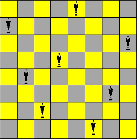
An 8-queen problem would the best example to use to illustrate here.  The goal of the 8-queens problem is to place eight queens on a chessboard such that no queen attacks any other. 

The best algorithm for solving this problem would be the min-conflicts heuristic repair method. The characteristics of the algorithm is to firstly repair inconsistencies in the current configuration, and then select a new value for a variable that results in the minimum number of conflicts with other variables. 

Detailed Steps: 

1. One by one, find out the number of conflicts between the inconsistent variable and other variables. 
2. Choose the one with the smallest number of conflicts to make a move. 
3. Repeat previous steps until all the inconsistent variables have been assigned with a proper value. 

         To apply these steps on an example from Pg. 114 of the textbook Artificial Intelligence: A Modern Approach,
         Stuart Russell - Peter Norvig - 1995.
 
 

State I                                     State II                                    State III 

 

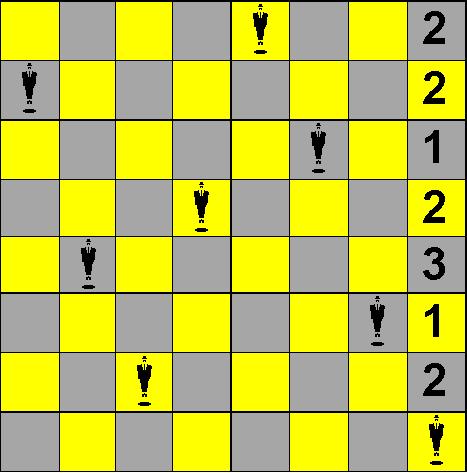
In State I, the 2 queens on fourth and eighth rows are attacking each other.  To find a new position for the eighth queen, we need to firstly find out the number of conflicts between this queen and all other queens.  The numbers of conflicts would be the numbers shown on the eighth column in State I. Why the number on the first row is two?  It is because that if we move the eighth queen up to the first row, there will be two other queens, one on the first row and the other on the third row, attacking it.  And so on for the rest positions. 

Now we are to choose a position with the smallest number of conflicts to place the eighth queen. The fact is that it is possible to have more than one best choice. The third row with one conflict would our choice for convenience. 

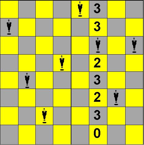
Then we have moved over to State II.  Since the eighth queen had moved to the third queen's position, we now need to look for a new position for the third queen.  So again, we repeat finding out the numbers of attacking queens to this third queen.  As same as above, the numbers of conflicts would be the numbers shown on the sixth column in State II.  The number three is on the first row because that if we move the third queen up to the first row, there will be three other queens, one on the first row, second on the fifth row, third on the third row (the originally eighth queen), attacking it. And so on for the rest positions.  But obviously, the last row would be the only best choice because it is the only one has no conflict.  Therefore, we move the third queen down to the last row, then we have found the optimal solution. 

This min-conflicts heuristic repair method has been proved to be surprisingly effective.  We have just seen how it can solve the above problem in two steps.  And it has been recorded to be able to solve a million-queens problem in an average of less than 50 steps.
 
 

Russel, S. and P. Norvig (1995). Artificial Intelligence - A Modern Approach.
Upper Saddle River, NJ, Prentice Hall.